In ggplot2, the function call aes() stands for aesthetic mapping—it’s how you tell ggplot which variables in your data should control which visual properties of the plot.
1. What “aesthetics” can you map?
| Aesthetic | Inside aes() you’d write… | What it does |
|---|---|---|
| x‐position | aes(x = some_variable) | Puts points along the horizontal axis |
| y‐position | aes(y = some_variable) | Puts points along the vertical axis |
| color | aes(colour = some_variable) | Varies point colors by levels or values |
| size | aes(size = some_variable) | Varies point size by values |
| shape | aes(shape = some_variable) | Uses different point shapes for categories |
| fill | aes(fill = some_variable) | Fills shapes (e.g. bars) with variable‐driven color |
Anything you want driven by your data goes inside aes().
2. Inside vs. outside aes()
-
Inside
aes()→ data‐drivengeom_point(aes(colour = species, size = cty))“Colour each point by its species; size each point by the
ctyvalue.” -
Outside
aes()→ fixed settinggeom_point(aes(colour = species), size = 3, alpha = 0.7)“Colour by species, but make every point size 3 and 70% opaque.”
3. Why is it necessary?
Without aes(), ggplot has no instruction about which column should control which visual channel. It would just plot all points in default color and size:
# No aes: every point identical
ggplot(mpg) +
  geom_point()
By adding aes(x, y), you map your data onto the axes:
ggplot(mpg, aes(x = hwy, y = displ)) +
  geom_point()
Now each point’s horizontal position comes from hwy and vertical from displ.
4. Common mistake: mapping the wrong type
geom_point(aes(shape = cty))If cty is continuous (many unique numbers), you’ll get:
✖ A continuous variable cannot be mapped to the shape aesthetic.
Because shapes are discrete categories—only a handful of glyphs are available. To fix, either:
-
Remove shape mapping
-
Convert to factor:
aes(shape = factor(cty)) -
Or use a different aesthetic (e.g.,
size)
5. Quick recipe
-
Decide which variable you want to control a visual property.
-
Put that mapping inside
aes(). -
Set any constant styling (size, alpha, color overrides) outside
aes().
Key takeaway:
aes()is the wiring harness between your raw data and the visual elements of your plot. Without it, ggplot doesn’t know what drives where or how to draw.
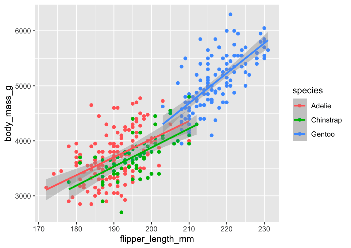
🖼️ Plot 1 – Multiple Lines (One per Species)
ggplot(
  data = penguins,
  mapping = aes(x = flipper_length_mm, y = body_mass_g, color = species)
) +
  geom_point() +
  geom_smooth(method = "lm")
What happens here:
-
color = speciesis defined globally. -
This means both:
-
The points are colored by species ✅
-
The lines are also colored by species ❗
-
-
So,
geom_smooth()draws one line per species.
📊 You get: 3 regression lines (1 for each species), each in a different color.
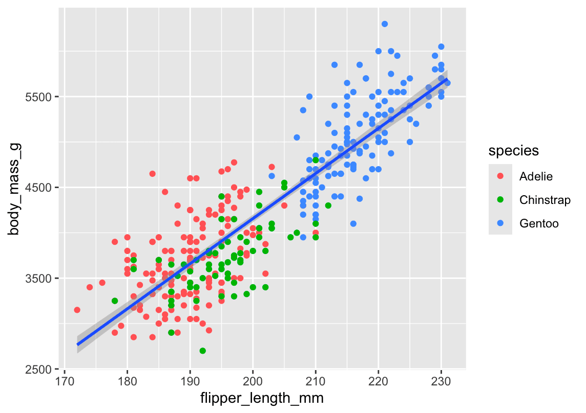
🖼️ Plot 2 – Single Line (All Species Together)
ggplot(
  data = penguins,
  mapping = aes(x = flipper_length_mm, y = body_mass_g)
) +
  geom_point(mapping = aes(color = species)) +
  geom_smooth(method = "lm")
What changes:
-
color = speciesis now insidegeom_point()only. -
So:
-
The points are still colored by species ✅
-
The line is drawn once for all data ❗ (no grouping by species)
-
📊 You get: 1 regression line, using all data regardless of species.
🧠 Quick Rule to Remember:
Where is color = species? | What you get |
|---|---|
Global (in ggplot()) | Colors everything (points & lines) = ➕ grouped smooth lines |
Local (in geom_point()) | Only colors the points = ➕ one unified line |
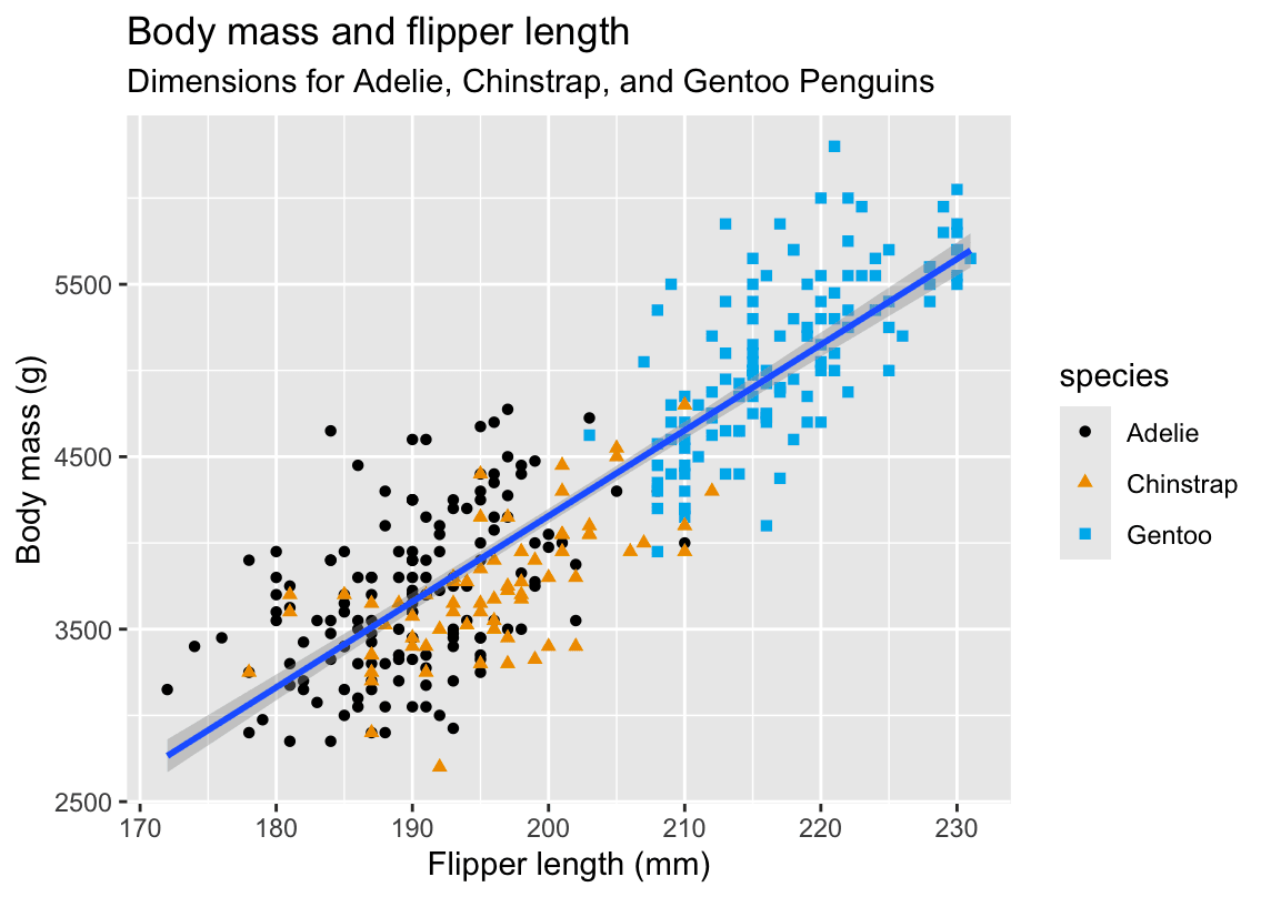
ggplot(
  data = penguins,
  mapping = aes(x = flipper_length_mm, y = body_mass_g)
) +
  geom_point(aes(color = species, shape = species)) +
  geom_smooth(method = "lm") +
  labs(
    title = 'Body mass and flipper length',
    subtitle = 'Dimensions for Adelie, Chinstrap, and Gentoo Penguins',
    x = "Flipper length (mm)", y = "Body mass (g)",
    color = 'species',shape='species'
  ) +
  scale_color_colorblind()
I asked AI to organize the notes based on my solution:
1.2.5 Exercises (palmerpenguins)
1. How many rows and columns are in penguins?
nrow(penguins)  # number of observations (rows)
ncol(penguins) # number of variables (columns)-
Answer:
-
Rows:
nrow(penguins) -
Columns:
ncol(penguins)
-
2. What does bill_depth_mm describe?
?penguins- Description:
bill_depth_mm= depth of the penguin’s bill (beak) in millimeters, measured at the thickest point.
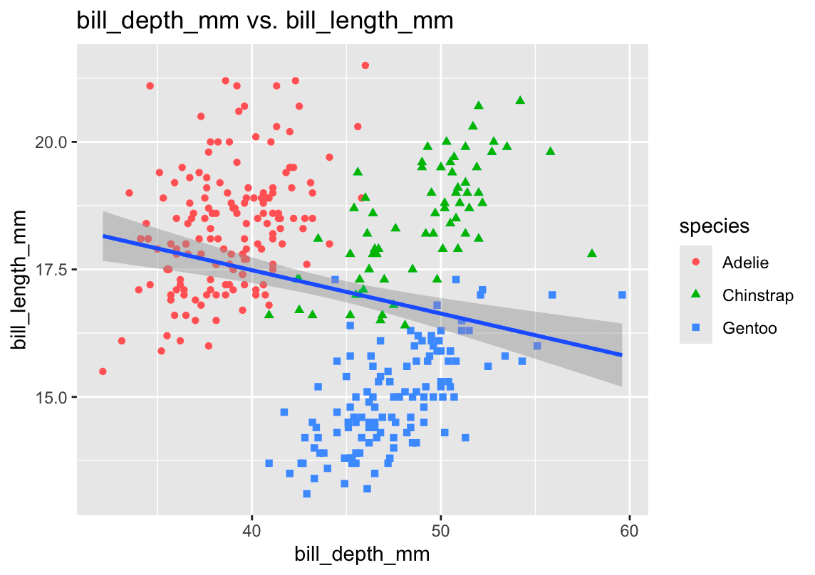
3. Scatterplot: bill_depth_mm vs. bill_length_mm
library(ggplot2)

ggplot(penguins, aes(x = bill_length_mm, y = bill_depth_mm)) +
  geom_point(aes(color = species, shape = species), alpha = 0.7) +
  geom_smooth(method = "lm", se = FALSE) +
  labs(
    title = "Bill Depth vs. Bill Length by Species",
    x     = "Bill Length (mm)",
    y     = "Bill Depth (mm)",
    color = "Species",
    shape = "Species"
)- Relationship:
There’s a moderate positive correlation—penguins with longer bills also tend to have deeper bills. Patterns differ by species.
4. Scatterplot of species vs. bill_depth_mm
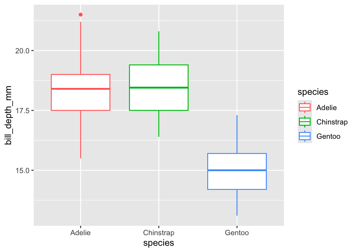
ggplot(penguins, aes(x = species, y = bill_depth_mm)) +
  geom_boxplot(aes(color = species)) +
  labs(
    title = "Distribution of Bill Depth by Species",
    x     = "Species",
    y     = "Bill Depth (mm)"
)-
What happens:
A plain scatter (geom_point) stacks points and overlaps heavily. -
Better choice:
geom_boxplot()(orgeom_violin()) to summarize each species’ distribution. but actually answer belike: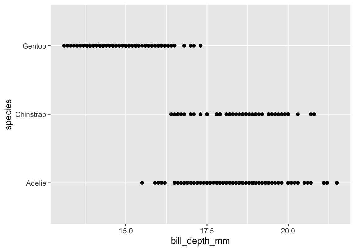
ggplot(
  data = penguins,
  aes(x = bill_depth_mm, y = species)
) +
  geom_point()
5. Why does this give an error?
ggplot(data = penguins) +
geom_point()-
Error:
geom_point()needs at leastaes(x, y); none were provided. -
Fix:
Supply aesthetics, for example:ggplot(penguins, aes(x = bill_length_mm, y = bill_depth_mm)) + geom_point()
6. The na.rm argument in geom_point()
-
What it does:
na.rm = TRUEremoves any rows withNAin the mapped aesthetics before plotting. -
Default:
na.rm = FALSE(will warn or drop NAs with a message).
ggplot(penguins, aes(x = bill_length_mm, y = bill_depth_mm)) +
  geom_point(na.rm = TRUE) +
  labs(
    title    = "Bill Measurements (NAs removed)",
    subtitle = "Using na.rm = TRUE",
    x        = "Bill Length (mm)",
    y        = "Bill Depth (mm)"
  )
7. Add a caption
Use labs(caption = "…"), for example:
+ labs(caption = "Data come from the palmerpenguins package.")8. Recreate this visualization
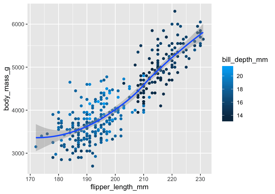
Task: scatterplot of body_mass_g vs flipper_length_mm, colored by bill_depth_mm, with a smooth curve.
ggplot(penguins, aes(x = flipper_length_mm, y = body_mass_g)) +
  geom_point(aes(color = bill_depth_mm), size = 2, alpha = 0.8) +
  geom_smooth(se = TRUE) +
  labs(
    title = "Body Mass vs. Flipper Length",
    x     = "Flipper Length (mm)",
    y     = "Body Mass (g)",
    color = "Bill Depth (mm)",
    caption = "Data come from the palmerpenguins package."
)-
Aesthetic mapping:
bill_depth_mm→ color, at thegeom_point()level (so the smooth line isn’t colored).
9. Predict the output of:
ggplot(
  data = penguins,
  mapping = aes(x = flipper_length_mm, y = body_mass_g, color = island)
) +
  geom_point() +
geom_smooth(se = FALSE)-
Prediction:
-
Points colored by
island. -
One smooth curve per island (because the color grouping is inherited), no confidence band.
-
10. Will these two graphs look different?
# A
ggplot(
  data = penguins,
  mapping = aes(x = flipper_length_mm, y = body_mass_g)
) +
  geom_point() +
  geom_smooth()

# B
ggplot() +
  geom_point(
    data = penguins,
    mapping = aes(x = flipper_length_mm, y = body_mass_g)
  ) +
  geom_smooth(
    data = penguins,
    mapping = aes(x = flipper_length_mm, y = body_mass_g)
)-
Answer: No—they’ll be identical.
-
In A, you set
dataandaesglobally. -
In B, you repeat them in each layer.
-
Result: same points + same smooth line with CI.
-
✅ Key Takeaways
-
Always check your axis labels match your
aes(x, y). -
Use boxplots or violins when plotting a continuous against a categorical variable.
-
Remember to supply
aes(x, y)or you’ll get an error. -
na.rm = TRUEquietly drops missing values. -
Captions live in
labs(caption = "..."). -
Map continuous color scales at the geom level if you don’t want the grouping applied to other geoms.
-
Global vs. per-layer
data/aesis purely syntactic—plots only care about the final mapping.
1.4 Visualizing distributions
1.4.1 A categorical variable
A variable is categorical if it can only take one of a small set of values. To examine the distribution of a categorical variable, you can use a bar chart.
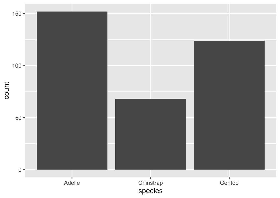
ggplot(penguins, aes(x = species)) +
  geom_bar()
t’s often preferable to reorder the bars based on their frequencies. Doing so requires transforming the variable to a factor (how R handles categorical data) and then reordering the levels of that factor.
fct_infreq() It reorders a factor based on how often each level occurs.
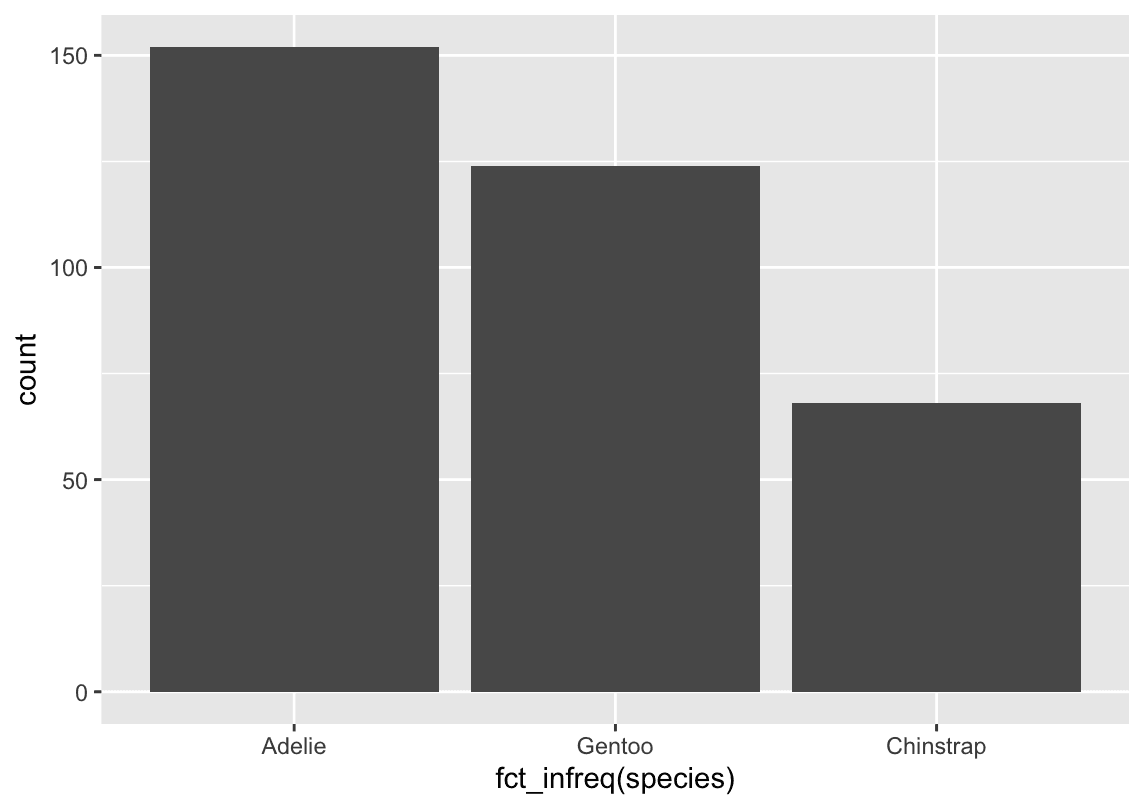
ggplot(penguins,aes(x = fct_infreq(species) )) +
  geom_bar()
1.4.2 A numerical variable
One commonly used visualization for distributions of continuous variables is a histogram. You should always explore a variety of binwidths when working with histograms, as different binwidths can reveal different patterns
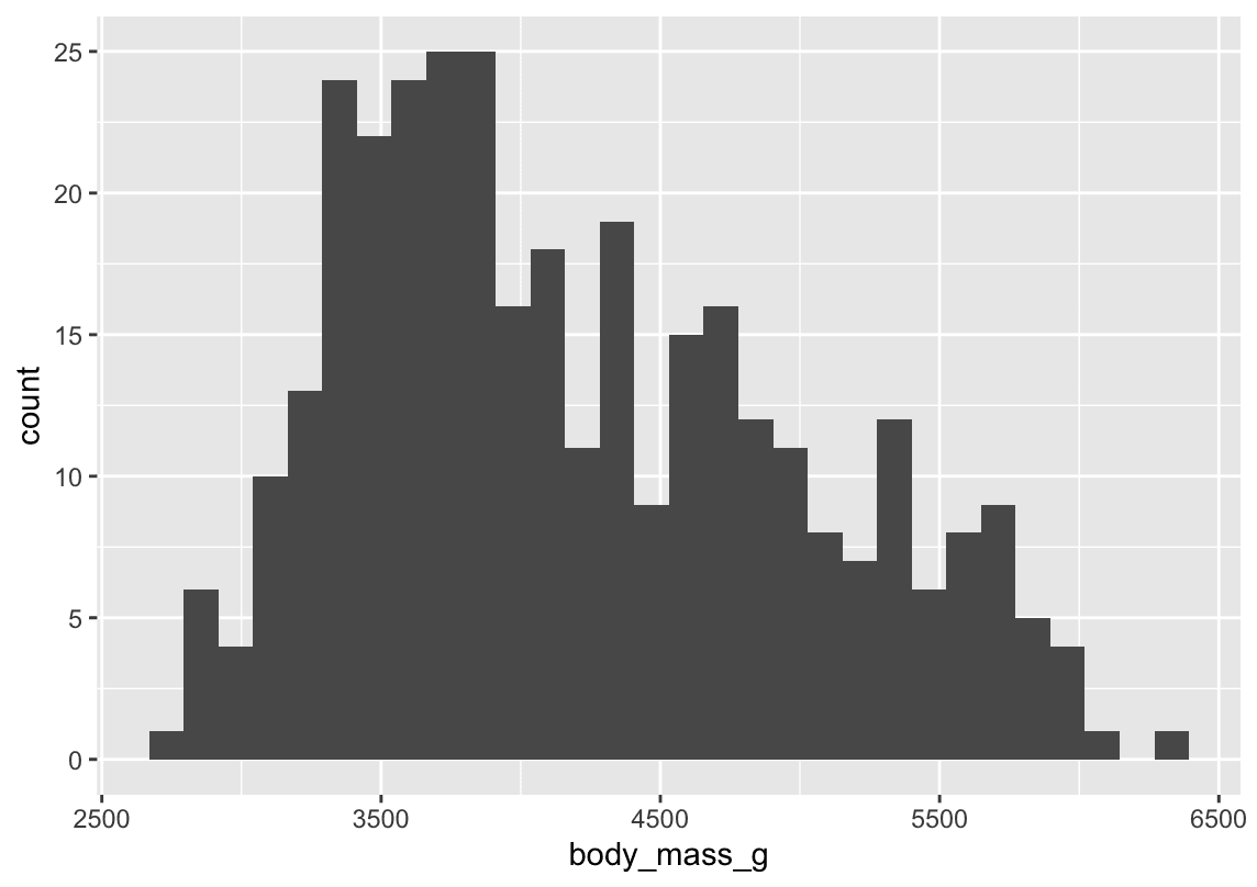
ggplot(penguins,aes(x=body_mass_g)) +
  geom_histogram()
An alternative visualization for distributions of numerical variables is a density plot.
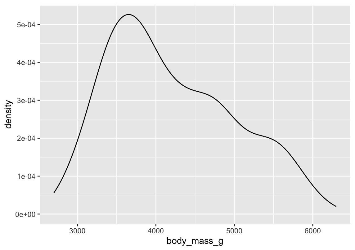
ggplot(penguins,aes(x=body_mass_g)) +
  geom_density()
1.4.3 Exercises
How are the following two plots different? Which aesthetic, color or fill, is more useful for changing the color of bars?
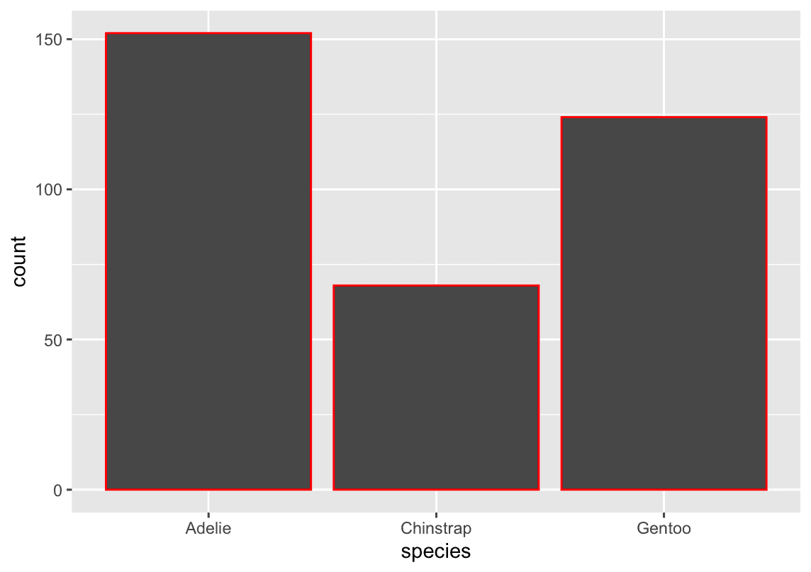
ggplot(penguins, aes(x = species)) +
  geom_bar(color = "red")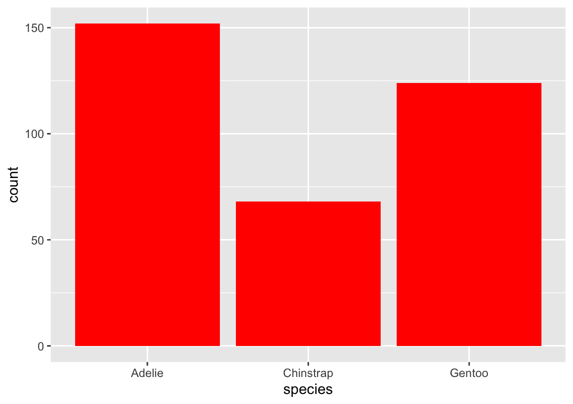
ggplot(penguins, aes(x = species)) +
  geom_bar(fill = "red")
1.5 Visualizing relationships
1.5.1 A numerical and a categorical variable
A boxplot is a type of visual shorthand for measures of position (percentiles) that describe a distribution.
ggplot(penguins,aes(x=species,y=body_mass_g)) +
  geom_boxplot()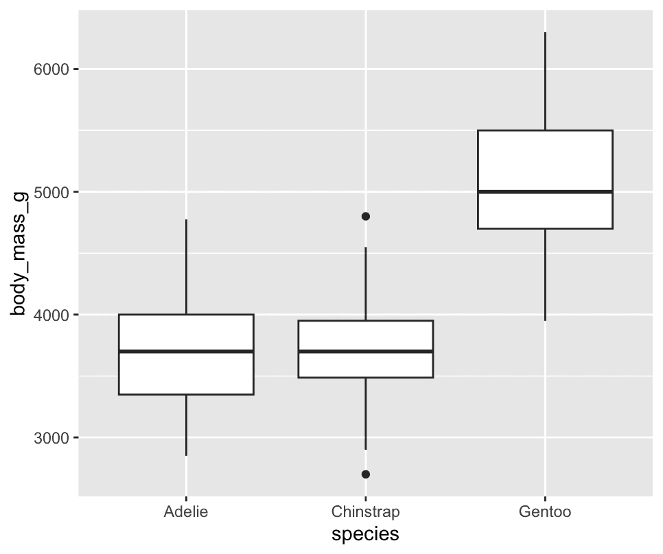
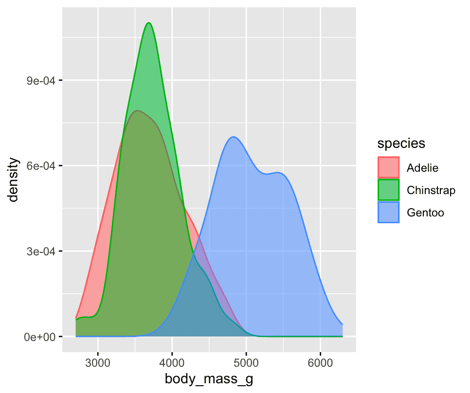
Alternatively, we can make density plots with `[geom_density()]
ggplot(penguins,aes(x=body_mass_g,colour = species, fill = species)) +
  geom_density(alpha=0.5)
1.5.2 Two categorical variables
We can use stacked bar plots to visualize the relationship between two categorical variables.
ggplot(penguins,aes(x=island,fill=species)) +
geom_bar()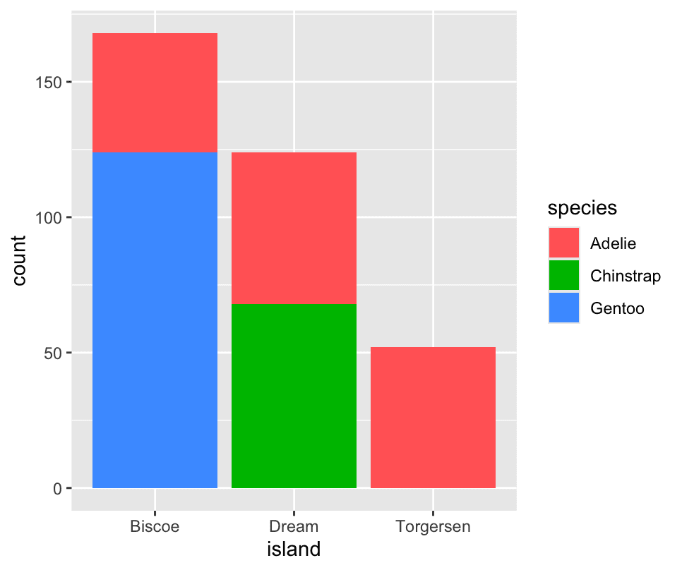 The second plot, a relative frequency plot
ggplot(penguins,aes(x=island,fill=species)) +
  geom_bar(position='fill')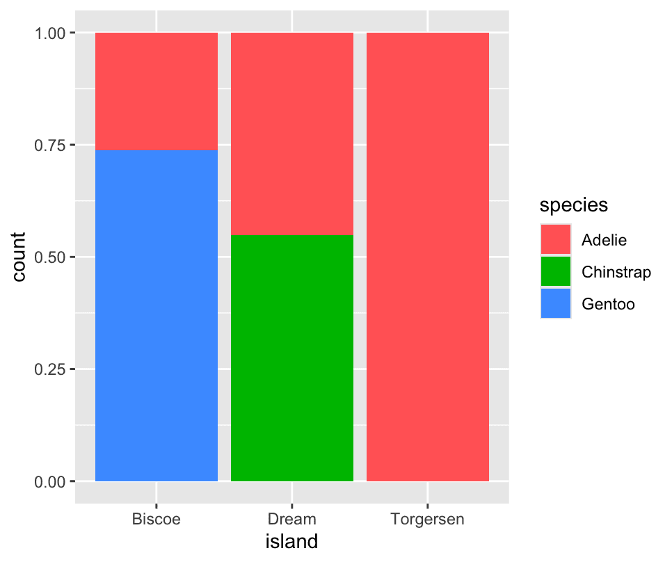
1.5.3 Two numerical variables
A scatterplot is probably the most commonly used plot for visualizing the relationship between two numerical variables.
ggplot(penguins, aes(x = flipper_length_mm, y = body_mass_g)) +
  geom_point()
Another way, which is particularly useful for categorical variables, is to split your plot into facets, subplots that each display one subset of the data.
To facet your plot by a single variable, use [facet_wrap()]. The first argument of [facet_wrap()] is a formula, which you create with ~ followed by a variable name. The variable that you pass to [facet_wrap()] should be categorical.
ggplot(penguins,aes(x=flipper_length_mm,y=body_mass_g)) +
  geom_point(aes(colour = species,shape = species)) +
  facet_wrap(~island)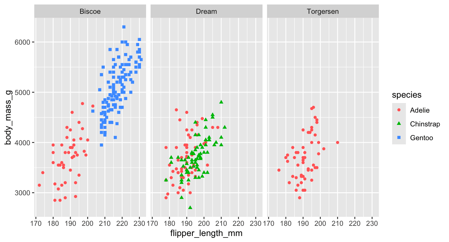
Why does the following yield two separate legends? How would you fix it to combine the two legends?
ggplot(
  data = penguins,
  mapping = aes(
    x = bill_length_mm, y = bill_depth_mm,
    color = species, shape = species
  )
) +
  geom_point() +
  labs(color = "Species")
In ggplot2, each aesthetic (colour, shape, size, fill, etc.) gets its own scale—and by default its own legend—because under the hood you have separate scales called scale_colour_discrete() and scale_shape_discrete(). Even if they’re mapped to the same variable, ggplot keeps them separate unless you explicitly give them the same name (and breaks).
Why you got two legends
-
You mapped species to both colour and shape.
-
You only renamed the colour legend via
labs(colour = "Species"). -
The shape scale was still using its default title (“species”), so ggplot treated them as two distinct legends.
How to merge them
You just need to give both scales the exact same name. ggplot will then automatically collapse them into a single legend:
ggplot(penguins, aes(
  x      = bill_length_mm,
  y      = bill_depth_mm,
  colour = species,
  shape  = species
)) +
  geom_point() +
  labs(
    colour = "Species",
    shape  = "Species"
  )
or equivalently
ggplot(penguins, aes(bill_length_mm, bill_depth_mm,
                     colour = species, shape = species)) +
  geom_point() +
  scale_colour_discrete(name = "Species") +
  scale_shape_discrete(name  = "Species")
What happens here
-
Both legends now have the title “Species”.
-
ggplot sees the same title and identical breaks (the same factor levels) on two discrete scales.
-
It merges them into one combined legend showing both the colour swatches and the shape glyphs under the single heading “Species.”
Quick recap
-
Separate legends appear whenever you map a variable to two different aesthetics but give them different scale names.
-
To combine legends, give both scales the same name (via
labs(),scale_*_discrete(name=…), orguides()).