9.2 Aesthetic mappings
Let’s start by visualizing the relationship between displ and hwy for various classes of cars. We can do this with a scatterplot where the numerical variables are mapped to the x and y aesthetics and the categorical variable is mapped to an aesthetic like color or shape.
ggplot(mpg,aes(x = displ, y = hwy, colour = class)) +
  geom_point()

ggplot(mpg,aes(x = displ,y = hwy, shape = class)) +
  geom_point()
#> Warning: The shape palette can deal with a maximum of 6 discrete values because more #> than 6 becomes difficult to discriminate #> ℹ you have requested 7 values. Consider specifying shapes manually if you #> need that many of them. #> Warning: Removed 62 rows containing missing values or values outside the scale range #> (`geom_point()`).

ggplot(mpg, aes(x = displ, y = hwy, size = class)) +
  geom_point()
#> Warning: Using size for a discrete variable is not advised.


ggplot(mpg, aes(x = displ, y = hwy, alpha = class)) +
  geom_point()
#> Warning: Using alpha for a discrete variable is not advised.
Mapping an unordered discrete (categorical) variable (class) to an ordered aesthetic (size or alpha) is generally not a good idea because it implies a ranking that does not in fact exist.
What happens if you map an aesthetic to something other than a variable name, like aes(color = displ < 5)? Note, you’ll also need to specify x and y.
gplot(mpg, aes(x = hwy, y = displ, color = displ < 5)) +
geom_point()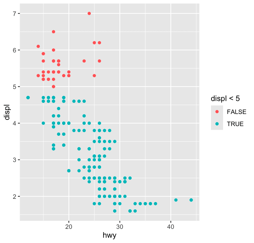 It creates a logical variable with values
 TRUE and FALSE for cars with displacement values below and above 5. In general, mapping an aesthetic to something other than a variable first evaluates that expression then maps the aesthetic to the outcome.
9.3 Geometric objects
Some aesthetics only apply to certain geoms. If you try to use an irrelevant one (like shape on a line), ggplot2 will ignore it. But when the aesthetic makes sense (like linetype for lines), ggplot2 uses it to distinguish different groups.
-
geom_smooth(),geom_line(), etc. need to know how to group data. -
If you map a discrete variable to an aesthetic like
colororlinetype, ggplot2 will:-
Automatically group the data by that variable
-
Add a legend
-
Use different visual styles ✅
-
-
If you only use
group, it will still draw the lines correctly, but without any visual or legend cue ❌
ggplot(mpg,aes(
  x = displ, y = hwy,
)) +
  geom_smooth(aes(group = drv))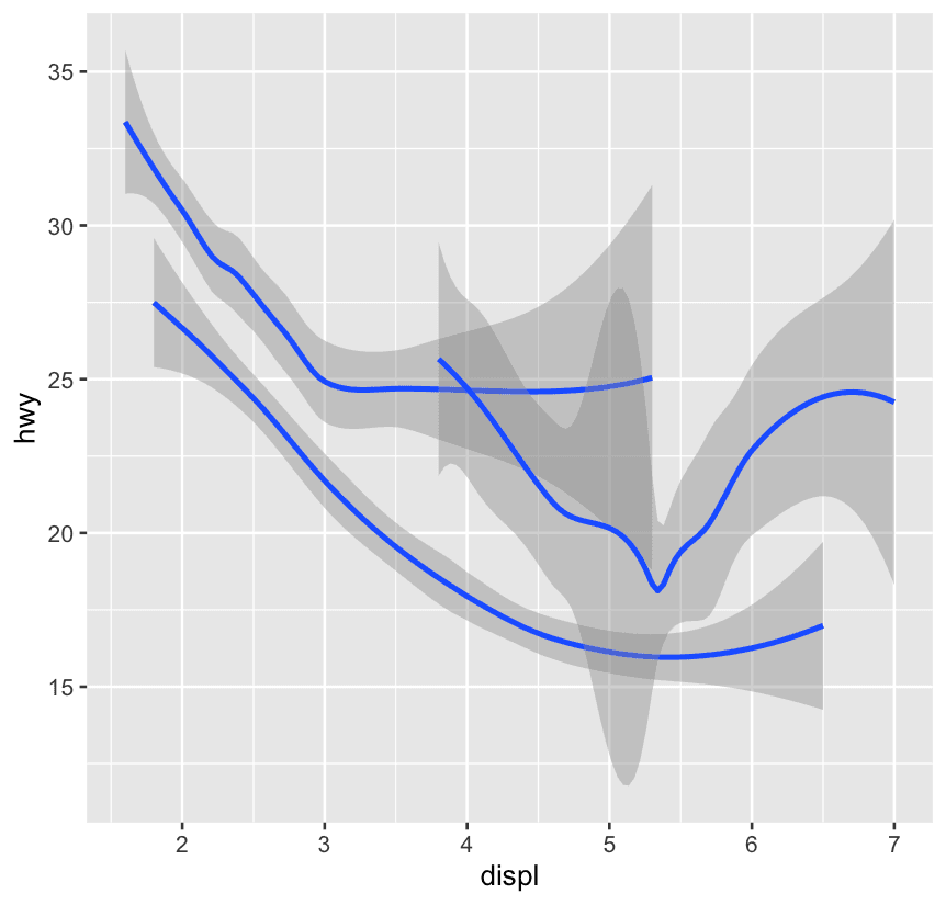
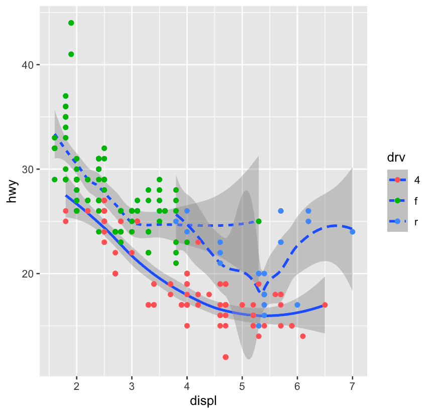
ggplot(mpg,aes(
  x = displ, y = hwy,
)) +
  geom_smooth(aes(color = drv))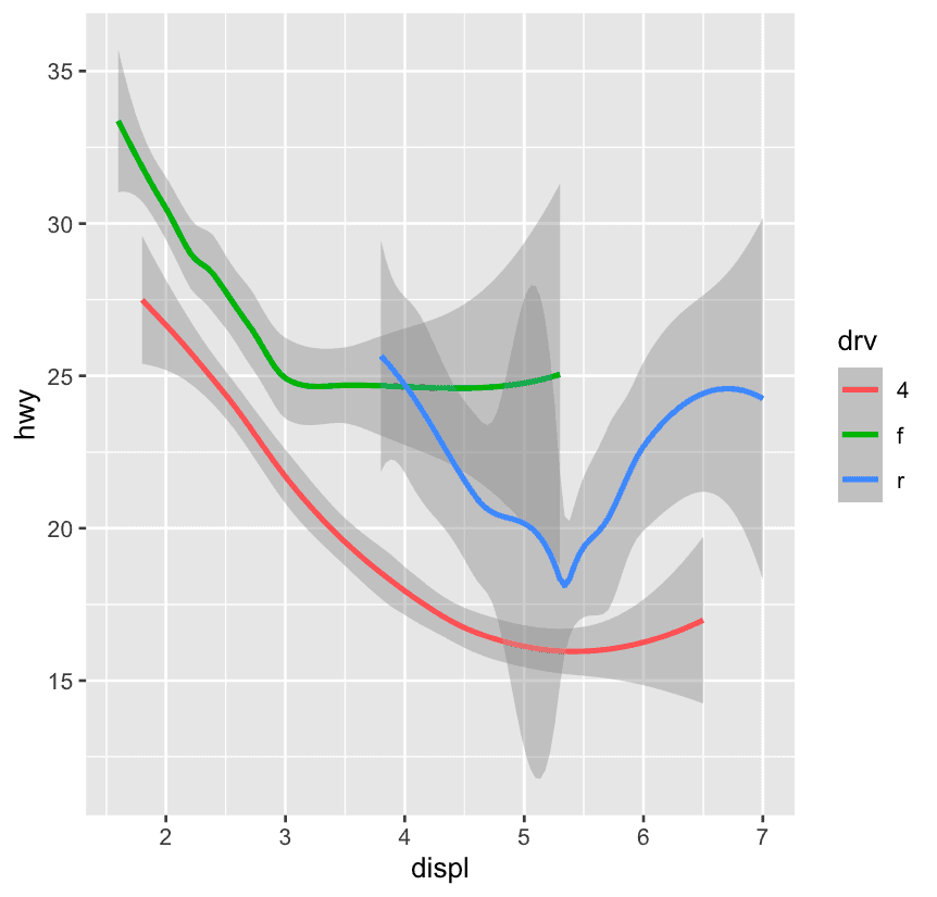
ggplot(mpg, aes(x = displ, y = hwy)) +
  geom_point() +
  geom_point(
    data = mpg |> filter(class == "2seater"),
    color = "red"
  ) + #Highlights the 2-seaters, but they **overlap** with the original black dots.
  geom_point(
    data = mpg |> filter(class == "2seater"),
    shape = "circle open", size = 3, color = "red"
  ) #This visually **outlines** the 2-seaters, giving them a "highlight ring" effect.
Think of ggplot2 like Photoshop layers:
-
First: black dots (all data)
-
Second: red dots (2seaters), but same size/shape — visually not clear
-
Third: open red circle — now they stand out clearly!
This pattern is useful for highlighting or annotating subsets without disturbing the main plot structure.
9.3.1 Exercises
ggplot(mpg,aes(
  x = displ, y = hwy, linetype = drv
)) +
  geom_smooth() +
  geom_point(aes(color = drv))
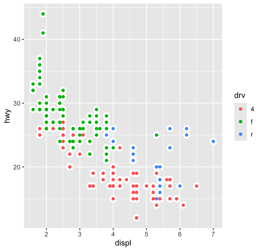
ggplot(mpg, aes(x = displ, y = hwy)) +
  geom_point(size = 4, color = "white") +
  geom_point(aes(color = drv))
9.4 Facets
faceting means you split your data into small multiples (subplots), each showing a different slice of your dataset.
1️⃣ facet_wrap(): one variable — like putting each “cookie tray” on a shelf
ggplot(mpg, aes(x = displ, y = hwy)) +
  geom_point() +
facet_wrap(~ class)-
This creates one plot per
classof car (like SUV, compact, etc.). -
It wraps the plots into a grid (usually fills rows first).
-
Only one variable used for facetting.
2️⃣ facet_grid(): two variables — like rows and columns of trays
ggplot(mpg, aes(x = displ, y = hwy)) +
  geom_point() +
facet_grid(drv ~ cyl)-
This makes a grid:
-
Rows =
drv(drive type: 4, f, r) -
Columns =
cyl(cylinder number)
-
-
It’s a two-sided formula:
rows ~ columns
3️⃣ Flexible Scales — to zoom in per plot
By default, facet_wrap() and facet_grid() use fixed axis scales. This is great for comparing, but…
Sometimes each plot has its own “story to tell,” and fixed scales make it hard to see!
Let’s fix that:
| Argument | What it does |
|---|---|
scales = "free" | both x and y axes vary |
scales = "free_x" | only x varies (across columns) |
scales = "free_y" | only y varies (across rows) |
ggplot(mpg, aes(x = displ, y = hwy)) +
  geom_point() +
  facet_wrap(~ class, scales = "free")
9.4.1 Exercises
What does . do?
with facet_grid(drv ~ .), the period means “don’t facet across columns”. In the second plot, with facet_grid(. ~ drv), the period means “don’t facet across rows”. In general, the period means “keep everything together”.
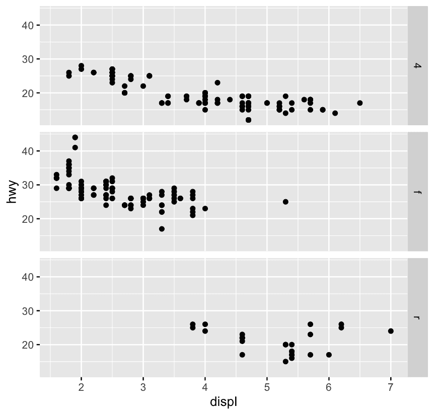
ggplot(mpg) +
  geom_point(aes(x = displ, y = hwy)) +
  facet_grid(drv ~ .)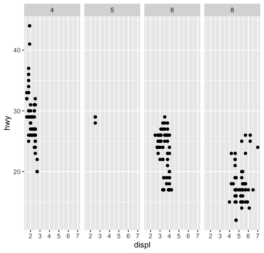
ggplot(mpg) +
  geom_point(aes(x = displ, y = hwy)) +
  facet_grid(. ~ cyl)
Which of the above plots makes it easier to compare engine size (displ) across cars with different drive trains? What does this say about when to place a faceting variable across rows or columns?
The first plot makes it easier to compare engine size (displ) across cars with different drive trains because the axis that plots displ is shared across the panels. What this says is that if the goal is to make comparisons based on a given variable, that variable should be placed on the shared axis.
9.5 Statistical transformations
ggplot(diamonds,aes(x = cut)) +
geom_bar()-
You pass the full
diamondsdataset. -
geom_bar()counts how many times eachcutappears. -
The y-axis is the frequency.
-
This is automatic summarization.
diamonds %>%
  count(cut) %>%
  ggplot(aes(x = cut,y = n)) +
geom_bar(stat = 'identity')-
You pre-counted the data using
count(cut). -
You explicitly mapped
y = n. -
You tell ggplot: “Just draw bars with height
n” — no counting. Imagine you’re building a shelf: -
If you just give a rough plan to a carpenter (like raw data), they’ll cut the wood for you → this is
stat = "count". -
But if you already have pre-cut wood pieces (like using
count()), you tell the carpenter “don’t cut anything, just use what I give you” → this isstat = "identity".
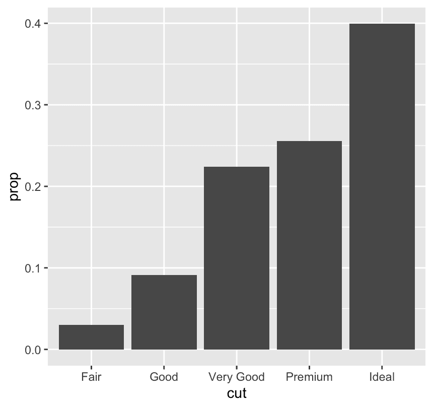
ggplot(diamonds,aes(x = cut,y = after_stat(prop),group = 1)) +
  geom_bar()
y = after_stat(prop)
after_stat(...)means:
“Use a variable that is computed by the stat (in this case,
stat_count(), the default stat forgeom_bar).”
propis one such computed value: it’s the proportion of the total count.
group = 1
This part is crucial!
Without it, ggplot would compute prop separately within each group — which could mess up the calculation.
By adding group = 1, you’re saying:
“Treat all the data as one group, so the proportions are relative to the entire dataset.”
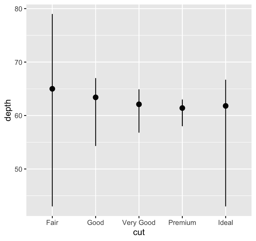
ggplot(diamonds) +
  stat_summary(
    aes(x = cut,y = depth),
    fun.min = min,
    fun.max = max,
    fun = median
  )
For each cut category, look at the depth values of the diamonds — and summarize them (using min, max, median).
| Argument | Purpose |
|---|---|
fun.min | Function to compute the bottom of the line segment (e.g., min()) |
fun.max | Function to compute the top of the line segment (e.g., max()) |
fun | Function to compute the center point (e.g., median()) |
stat_summary() doesn’t know how to summarize your data unless you tell it how. |
You’re answering:
-
Do I want the average? → use
fun = mean -
Do I want the median? → use
fun = median -
Do I want the maximum? → use
fun.max = max
Think of fun as the brain telling ggplot: what number to show per group.
9.6 Position adjustments
ggplot(mpg, aes(x = drv, color = drv)) +
geom_bar(linewidth = 1.2) 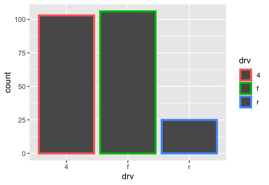
ggplot(mpg,aes(x=drv,fill = drv)) +
  geom_bar()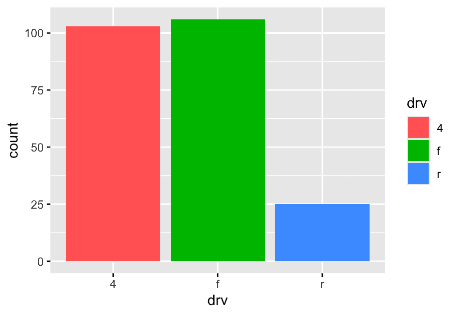
what happens if you map the fill aesthetic to another variable, like class: the bars are automatically stacked. Each colored rectangle represents a combination of drv and class
ggplot(mpg,aes(x=drv,fill = class)) +
  geom_bar()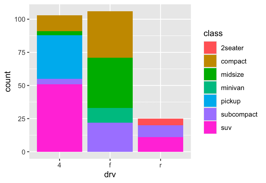
position = "fill"works like stacking, but makes each set of stacked bars the same height. This makes it easier to compare proportions across groups.
ggplot(mpg,aes(x = drv,fill = class)) +
  geom_bar(position = 'fill')
same as above
position = "dodge"places overlapping objects directly beside one another. This makes it easier to compare individual values.
ggplot(mpg,aes(x = drv,fill = class)) +
  geom_bar(position = 'dodge')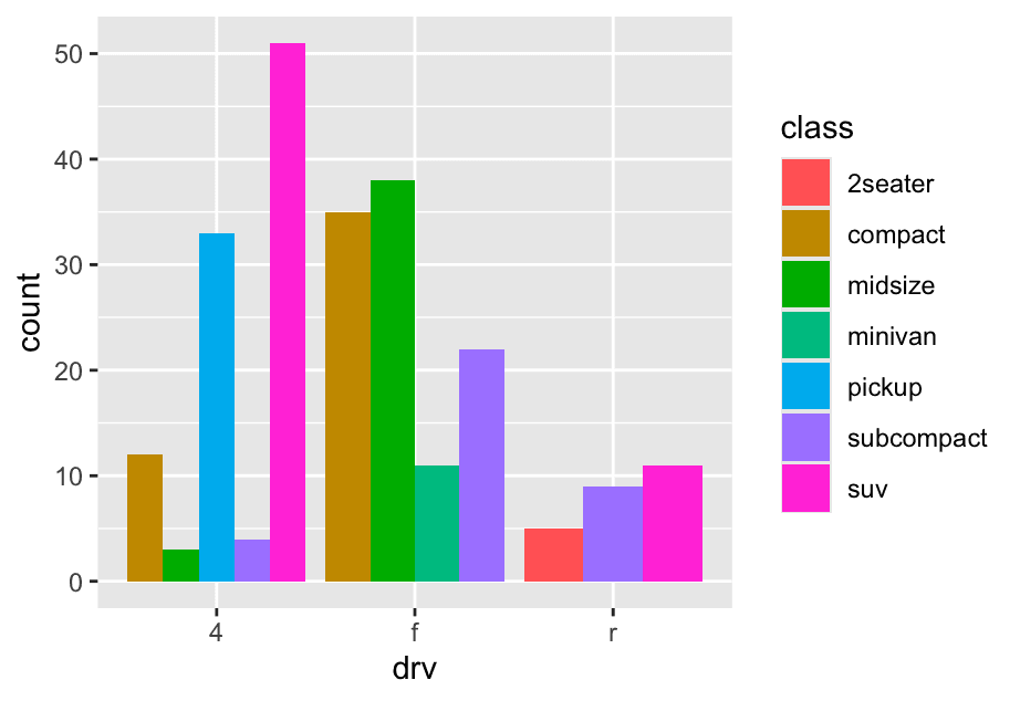
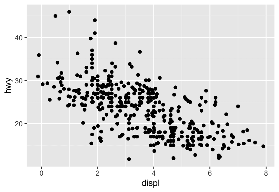
There’s one other type of adjustment that’s not useful for bar charts, but can be very useful for scatterplots. Recall our first scatterplot. Did you notice that the plot displays only 126 points, even though there are 234 observations in the dataset?
The underlying values of hwy and displ are rounded so the points appear on a grid and many points overlap each other. This problem is known as overplotting.
You can avoid this gridding by setting the position adjustment to “jitter”. position = "jitter" adds a small amount of random noise to each point. This spreads the points out because no two points are likely to receive the same amount of random noise.
ggplot(mpg,aes(x = displ,y = hwy)) +
geom_point(position = 'jitter')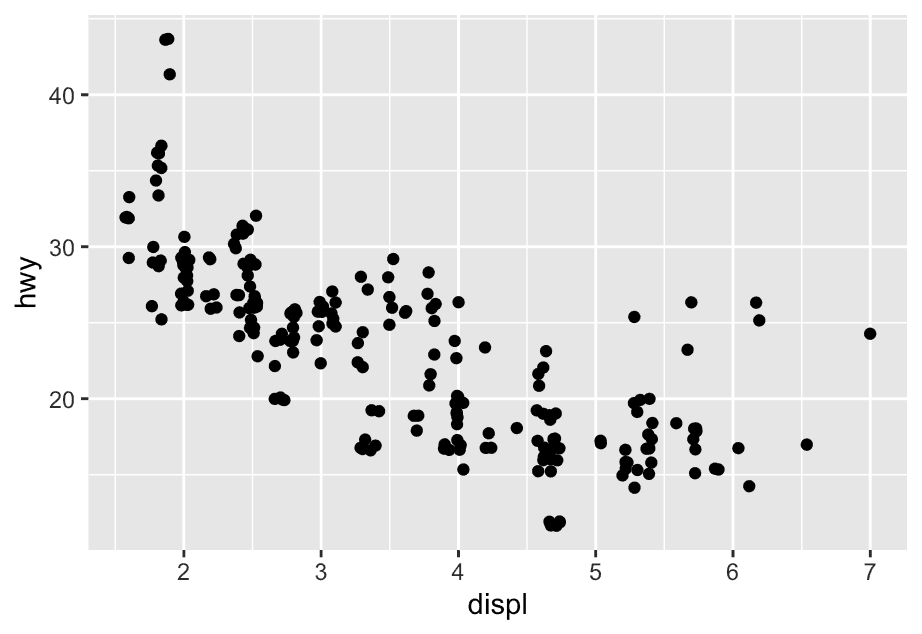 Adding randomness seems like a strange way to improve your plot, but while it makes your graph less accurate at small scales, it makes your graph more revealing at large scales.
9.6.1 Exercises
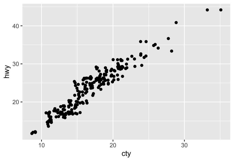
1 What is the problem with the following plot? How could you improve it?
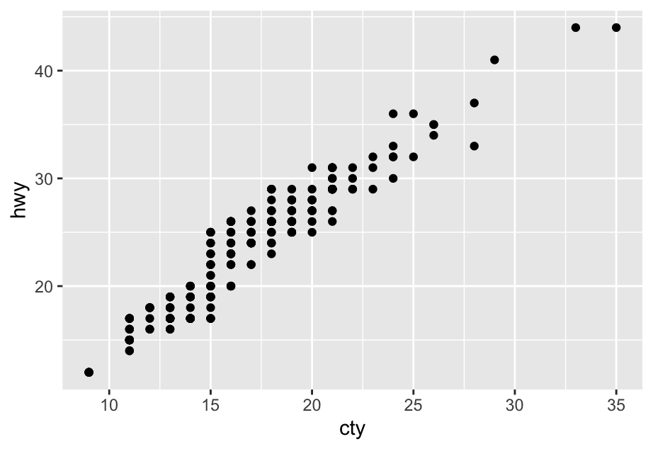
ggplot(mpg, aes(x = cty, y = hwy)) +
  geom_point()
The mpg dataset has 234 observations, however the plot shows fewer observations than that. This is due to overplotting; many cars have the same city and highway mileage. This can be addressed by jittering the points.
ggplot(mpg, aes(x = cty, y = hwy)) +
  geom_point()
2 What, if anything, is the difference between the two plots? Why?
ggplot(mpg, aes(x = displ, y = hwy)) +
  geom_point()
ggplot(mpg, aes(x = displ, y = hwy)) +
  geom_point(position = "identity")
The two plots are identical.
So what does position = "identity" mean?
It means:
Don’t adjust the position of elements — draw them exactly where they are.
In other words, just stack or place them as-is — no dodging, stacking, or adjusting to avoid overlap.
Let’s say you have two groups of bars at the same x-position:
df <- tibble(
  group = c("A", "A", "B", "B"),
  category = c("X", "Y", "X", "Y"),
  value = c(5, 3, 4, 6)
)

ggplot(df, aes(x = group, y = value, fill = category)) +
  geom_col(position = "identity")
In this case, both bars for "A" and "B" will overlap because you’re telling ggplot:
“Just plot them exactly where the data says, no adjustment.”
So it often looks messy or confusing unless you:
-
Use transparency (
alpha) to see overlaps. -
Or manually adjust x-positions.
3 What parameters to geom_jitter() control the amount of jittering?
The width and height parameters control the amount of horizontal and vertical displacement, recpectively. Higher values mean more displacement.
ggplot(mpg,aes(x = displ,y = hwy)) +
  geom_point() +
  geom_jitter(height = 2,width = 2)