Transform 13 Numbers

13.2 Making numbers

readr provides two useful functions for parsing strings into numbers: parse_double() and parse_number(). Use parse_double() when you have numbers that have been written as strings:

x <- c("1.2", "5.6", "1e3")
parse_double(x)

Use parse_number() when the string contains non-numeric text that you want to ignore. This is particularly useful for currency data and percentages:

x <- c("$1,234", "USD 3,513", "59%")
parse_number(x)

13.3 Counts

It’s surprising how much data science you can do with just counts and a little basic arithmetic, so dplyr strives to make counting as easy as possible with count(). This function is great for quick exploration and checks during analysis:

flights %>% 
  count(dest)

If you want to see the most common values, add sort = TRUE flights |> count(dest, sort = TRUE)

You can perform the same computation “by hand” with group_by(), summarize() and n(). This is useful because it allows you to compute other summaries at the same time:

flights %>% 
  group_by(dest) %>% 
  summarise(
    n = n(),
    delay = mean(arr_delay,na.rm = TRUE)
  )

n() is a special summary function that doesn’t take any arguments and instead accesses information about the “current” group. This means that it only works inside dplyr verbs

n_distinct(x) counts the number of distinct (unique) values of one or more variables. For example, we could figure out which destinations are served by the most carriers:

flights %>% 
  group_by(dest) %>% 
  summarise(
    carriers = n_distinct(carrier) 
  ) %>% 
  arrange(desc(carriers))

A weighted count is a sum. For example you could “count” the number of miles each plane flew:

flights |> 
  group_by(tailnum) |> 
  summarize(miles = sum(distance))

A normal count is just how many times something appears.
A weighted count is a sum of weights (like distance, cost, or time) associated with each item — not just how many times it appears.

You can count missing values by combining sum() and is.na(). In the flights dataset this represents flights that are cancelled:

flights %>% 
  group_by(dest) %>% 
  summarise(
    cancelled = sum(is.na(dep_time))
  )

How can you use count() to count the number of rows with a missing value for a given variable? Suppose you want to know: How many rows have a missing value (NA) in the dep_time column of flights?

flights %>% 
  count(is.na(dep_time))

13.4 Numeric transformations

13.4.1 Arithmetic and recycling rules

1. What is Vector Recycling in R?

Vector recycling means:
When you do operations with two vectors of different lengths, R “repeats” (recycles) the shorter vector until it matches the length of the longer one.

Example:
Let’s say you have

x <- c(1, 2, 10, 20)

And you multiply by a shorter vector:

x * c(1, 2)

What happens?

R takes c(1, 2) and recycles it, making it [1, 2, 1, 2] to match the length of x.
So, the calculation is:
- 1 * 1 = 1
- 2 * 2 = 4
- 10 * 1 = 10
- 20 * 2 = 40

Result:

[1]  1  4 10 40

2. What if lengths don’t “fit”?

If the long vector’s length is not a multiple of the short one, R still tries to recycle — but gives you a warning.

x * c(1, 2, 3)

x has length 4.
c(1, 2, 3) gets recycled as [1, 2, 3, 1]
Calculation:
- 1 * 1 = 1
- 2 * 2 = 4
- 10 * 3 = 30
- 20 * 1 = 20

R gives a warning because 4 (length of x) isn’t a multiple of 3.

3. Logical Comparisons and Recycling

This recycling also happens with logical comparisons (==, <, etc.).

Why is this dangerous?
If you accidentally use == with a vector instead of %in%, recycling happens and gives you results you don’t expect.

4. A Common Mistake in Filtering DataFrames

You want all flights in January or February.
Many people write:

flights |> filter(month == c(1, 2))

BUT:

month == c(1, 2) uses recycling.
R compares first row’s month with 1, second row’s month with 2, third with 1, fourth with 2, etc.

Result:

Odd rows: Checks if month == 1
Even rows: Checks if month == 2

If your dataframe has an even number of rows, there’s no warning.
But you’re not getting “all January and February flights”—you’re getting a weird mix based on row position!

🔑 Key Takeaway

Whenever you want to check if a value matches any of several options in R, use %in% instead of ==.

13.4.2 Minimum and maximum

The arithmetic functions work with pairs of variables. Two closely related functions are pmin() and pmax(), which when given two or more variables will return the smallest or largest value in each row:

 
df <- tribble(
  ~x, ~y,
  1,  3,
  5,  2,
  7, NA,
)
 
df %>% 
  mutate(
    min = pmin(x,y,na.rm = TRUE),
    max = pmax(x,y,na.rm = TRUE)
  )
# A tibble: 3 × 4
      x     y   min   max
  <dbl> <dbl> <dbl> <dbl>
1     1     3     1     3
2     5     2     2     5
3     7    NA     7     7

Note that these are different to the summary functions min() and max() which take multiple observations and return a single value

df |> 
  mutate(
    min = min(x, y, na.rm = TRUE),
    max = max(x, y, na.rm = TRUE)
  )
#> # A tibble: 3 × 4
#>       x     y   min   max
#>   <dbl> <dbl> <dbl> <dbl>
#> 1     1     3     1     7
#> 2     5     2     1     7
#> 3     7    NA     1     7

13.4.3 Modular arithmetic

In R, %/% does integer division and ` 100, .keep = ‘used’ )


We can combine that with the `mean(is.na(x))` trick to see how the proportion of cancelled flights varies over the course of the day.
```r
flights %>% 
  group_by(hour = sched_dep_time %/% 100) %>% 
  summarise(
    proportion_cancelled = mean(is.na(dep_time)),
    n = n()
  ) %>% 
  filter(hour > 1) %>% 
  ggplot(aes(x = hour,y = proportion_cancelled)) +
  geom_line() +
  geom_point(aes(size = n))

is.na(dep_time) checks if each flight was cancelled (TRUE if cancelled, FALSE if not).
In R, TRUE is counted as 1, and FALSE as 0.
mean(is.na(dep_time)) adds up all the 1’s and 0’s, then divides by the total number of flights—so it gives you the proportion of cancelled flights (the fraction that are cancelled).
Only keep hours after 1 AM—usually because there are very few or no flights at 0 or 1 AM, which could make the plot misleading.
geom_point(aes(size = n)): Draws points at each hour, where the size of the point represents the number of flights scheduled in that hour. Bigger points = more flights.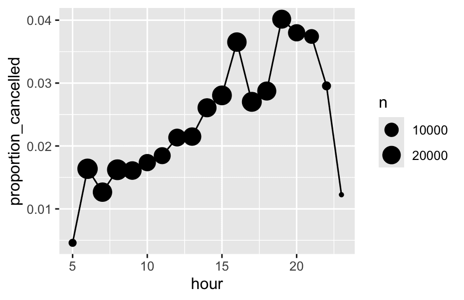

13.4.5 Rounding

Use round(x) to round a number to the nearest integer

You can control the precision of the rounding with the second argument, digits. round(x, digits) rounds to the nearest 10^-n so digits = 2 will round to the nearest 0.01. This definition is useful because it implies round(x, -3) will round to the nearest thousand, which indeed it does:

round(123.456, 2)  # two digits
#> [1] 123.46
round(123.456, 1)  # one digit
#> [1] 123.5
round(123.456, -1) # round to nearest ten
#> [1] 120
round(123.456, -2) # round to nearest hundred
#> [1] 100

if a number is half way between two integers, it will be rounded to the even integer.

> round(3.5)
[1] 4
> round(4.5)
[1] 4

round() is paired with floor() which always rounds down and ceiling() which always rounds up

These functions don’t have a digits argument, so you can instead scale down, round, and then scale back up:

floor(123.4567 / 0.01) * 0.01
ceiling(x / 0.01) * 0.01

13.4.6 Cutting numbers into ranges

Use cut()to break up (aka bin) a numeric vector into discrete buckets:

x <- c(1, 2, 5, 10, 15, 20)
cut(x,breaks = c(0,5,10,100))

You can optionally supply your own labels. Note that there should be one less labels than breaks.

cut(x, 
  breaks = c(0, 5, 10, 15, 20), 
  labels = c("sm", "md", "lg", "xl")
)
#> [1] sm sm sm md lg xl
#> Levels: sm md lg xl

13.4.7 Cumulative and rolling aggregates

Base R provides cumsum(), cumprod(), cummin(), cummax() for running, or cumulative, sums, products, mins and maxes. dplyr provides cummean() for cumulative means. Cumulative sums tend to come up the most in practice:

x <- 1:10
cumsum(x)

13.5 General transformations

Great, let’s break this down with simple explanations and analogies for each function!

13.5.1 Ranks

What’s a Ranking Function?

A ranking function assigns a position (1st, 2nd, 3rd, etc.) to each value in a list, based on its order.
This is useful when you want to know, for example, who has the highest score, or which value is in the top 10%.

1. min_rank()

Gives the “standard” ranks: lowest value is 1, next is 2, and so on.
Ties get the same rank, and the next rank is skipped.
- Example: 1st, 2nd, 2nd, 4th

x <- c(1, 2, 2, 3, 4, NA)
min_rank(x)
#> [1]  1  2  2  4  5 NA

NA stays NA.

2. desc(x)

Makes largest values get rank 1.

min_rank(desc(x))
#> [1]  5  3  3  2  1 NA

3. row_number()

Assigns a unique row number within ties (no skipped numbers).
- So, ties just get an arbitrary order.

row_number(x)  # [1] 1 2 3 4 5 NA

4. dense_rank()

Like min_rank(), but doesn’t skip numbers after ties.
- Example: 1st, 2nd, 2nd, 3rd (no jump)

dense_rank(x)  # [1] 1 2 2 3 4 NA

5. percent_rank()

Shows where each value falls as a percentage (0 to 1) of the way through the data.
0 = smallest, 1 = largest.

percent_rank(x)  # [1] 0.00 0.25 0.25 0.75 1.00 NA

6. cume_dist()

Cumulative proportion: For each value, what fraction of data is less than or equal to that value?
1 means the very top.

cume_dist(x)  # [1] 0.2 0.6 0.6 0.8 1.0 NA

13.5.2 Offsets

What do lag() and lead() do?

Imagine you have a list of numbers, like a time series or sequence:

x <- c(2, 5, 11, 11, 19, 35)
lag(x)
#> [1] NA  2  5 11 11 19
lead(x)
#> [1]  5 11 11 19 35 NA

lag(x): shifts everything down by one position—each value is replaced by the one before it. The first position becomes NA (nothing before it).
lead(x): shifts everything up by one position—each value is replaced by the one after it. The last position becomes NA (nothing after it).

In plain language:

lag(x): “What was the value just before this one?”
lead(x): “What will the value be just after this one?”
Great for finding changes, trends, or repeats in your data.

Why are they useful?

1. Calculate the change between values

If you want to see how much each value has changed compared to the previous one, you can do:

x - lag(x)
#> [1] NA  3  6  0  8 16

2. Detect when values stay the same (or change)

To find where the value repeats (stays the same as before):

x == lag(x)
#> [1]    NA FALSE FALSE  TRUE FALSE FALSE

This returns TRUE if the current value is the same as the previous value.

13.5.3 Consecutive identifiers

Why do we need consecutive identifiers?

Sometimes, you want to start a new group every time something changes (like a new session, or a new value appears in a sequence). This is different from just grouping by value, because the same value can appear in multiple, non-adjacent places, and each “run” should get its own group.

1. Grouping by gaps (sessions) using cumsum()

Suppose you have timestamps of web visits:

events <- tibble(time = c(0, 1, 2, 3, 5, 10, 12, 15, 17, 19, 20, 27, 28, 30))
events <- events %>% 
  mutate(
    diff = time - lag(time,default = first(time)),
    has_gap = diff >= 5
  )

You compute time difference with lag().
If the gap is big enough (e.g., diff >= 5), you set has_gap = TRUE.
lag(time) gives you the value from the previous row. For the first row, there is no previous value, so you use default = first(time) (which is just the first time value, usually 0).

Row	time	lag(time, default = 0)	diff (= time - lag(time))
1	0	0	0 - 0 = 0
2	1	0	1 - 0 = 1
3	2	1	2 - 1 = 1
4	3	2	3 - 2 = 1
…	…	…	…

Then:

events |> mutate(group = cumsum(has_gap))
# A tibble: 14 × 4
    time  diff has_gap group
   <dbl> <dbl> <lgl>   <int>
 1     0     0 FALSE       0
 2     1     1 FALSE       0
 3     2     1 FALSE       0
 4     3     1 FALSE       0
 5     5     2 FALSE       0
 6    10     5 TRUE        1
 7    12     2 FALSE       1
 8    15     3 FALSE       1
 9    17     2 FALSE       1
10    19     2 FALSE       1
11    20     1 FALSE       1
12    27     7 TRUE        2
13    28     1 FALSE       2
14    30     2 FALSE       2

Why use mutate(group = cumsum(has_gap))?

You want to split your timeline of events into sessions.
A new session starts every time there’s a big gap (has_gap == TRUE).
You need a column that tells you, for each event, which session it belongs to.
cumsum() (“cumulative sum”) increases by 1 every time has_gap is TRUE.
Result: Each “session” gets a unique group number!

2. Grouping by consecutive runs of values: consecutive_id()

Now suppose you have values that repeat, but not all together:

x = c("a", "a", "a", "b", "c", "c", "d", "e", "a", "a", "b", "b")

If you do group_by(x), all the “a”s will be grouped together, no matter where they appear.

But if you want to treat each consecutive “run” of the same value as a different group, use consecutive_id(x):

df |> 
  group_by(id = consecutive_id(x)) |> 
  slice_head(n = 1)

This will:

Assign a new group each time the value of x changes (not just each unique value).
So, the first three “a”s are group 1, the next “b” is group 2, and so on.

Result: You can grab, for example, the first row of each run.

Summary Table Example:

Suppose x =
a, a, a, b, c, c, d, e, a, a, b, b

row	x	id (consecutive_id)
1	a	1
2	a	1
3	a	1
4	b	2
5	c	3
6	c	3
7	d	4
8	e	5
9	a	6
10	a	6
11	b	7
12	b	7

Now, you can do things like:

Take the first or last row of each run.
Summarize statistics within each consecutive group.

🪴LYC