10.2 Questions

There is no rule about which questions you should ask to guide your research. However, two types of questions will always be useful for making discoveries within your data. You can loosely word these questions as:

1. What type of variation occurs within my variables?

2. What type of covariation occurs between my variables?

10.3 Variation

10.3.1 Typical values

In both bar charts and histograms, tall bars show the common values of a variable, and shorter bars show less-common values. Places that do not have bars reveal values that were not seen in your data. To turn this information into useful questions, look for anything unexpected:

• Which values are the most common? Why?

• Which values are rare? Why? Does that match your expectations?

• Can you see any unusual patterns? What might explain them?

ggplot(diamonds,aes(x = carat)) +
  geom_histogram(binwidth = 0.6)

smaller <- diamonds %>% 
  filter(carat < 3)
 
ggplot(smaller, aes(x = carat)) +
  geom_histogram(binwidth = 0.05)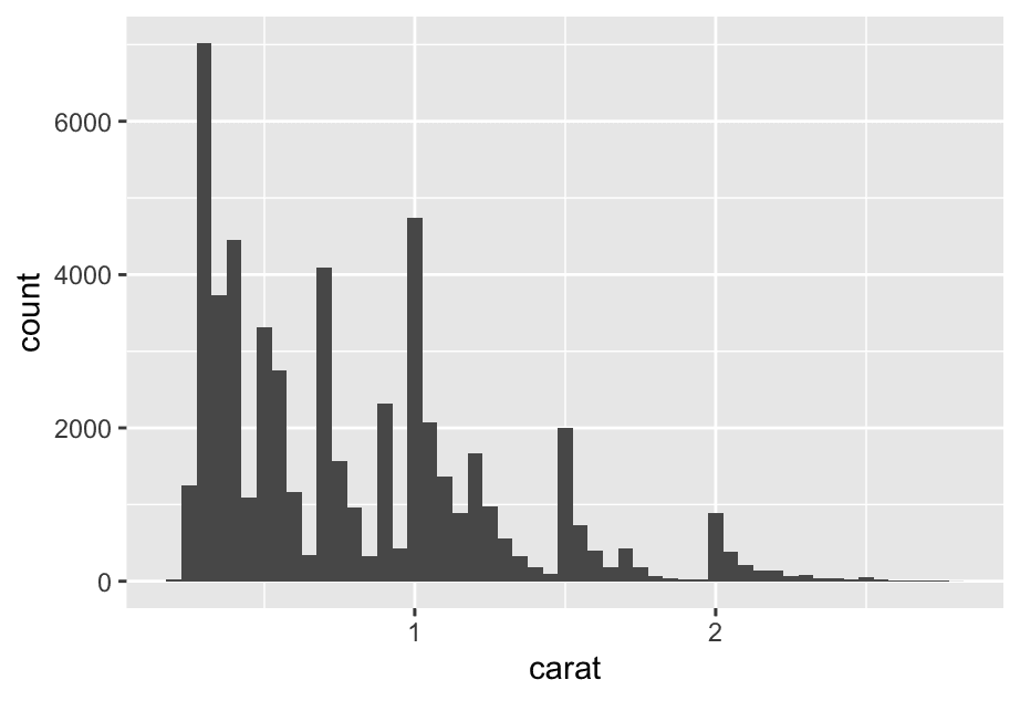

This histogram suggests several interesting questions:

• Why are there more diamonds at whole carats and common fractions of carats?

• Why are there more diamonds slightly to the right of each peak than there are slightly to the left of each peak?

Visualizations can also reveal clusters, which suggest that subgroups exist in your data. To understand the subgroups, ask:

• How are the observations within each subgroup similar to each other?

• How are the observations in separate clusters different from each other?

• How can you explain or describe the clusters?

• Why might the appearance of clusters be misleading?

10.3.2 Unusual values

ggplot(diamonds, aes(x = y)) + 
  geom_histogram(binwidth = 0.5)

To make it easy to see the unusual values, we need to zoom to small values of the y-axis with coord_cartesian():

ggplot(diamonds,aes(x = y)) +
  geom_histogram(binwidth = 0.5) +
  coord_cartesian(ylim = c(0,50))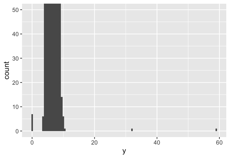

This allows us to see that there are three unusual values: 0, ~30, and ~60. We pluck them out with dplyr:

unusual <- diamonds %>% 
  filter(y < 3 | y > 20) %>% 
  select(price, x, y, z) %>% 
  arrange(y)
unusual
A tibble: 9 × 4
  price     x     y     z
  <int> <dbl> <dbl> <dbl>
1  5139  0      0    0   
2  6381  0      0    0   
3 12800  0      0    0   
4 15686  0      0    0   
5 18034  0      0    0   
6  2130  0      0    0   
7  2130  0      0    0   
8  2075  5.15  31.8  5.12
9 12210  8.09  58.9  8.06

The y variable measures one of the three dimensions of these diamonds, in mm. We know that diamonds can’t have a width of 0mm, so these values must be incorrect. By doing EDA, we have discovered missing data that was coded as 0, which we never would have found by simply searching for NAs. Going forward we might choose to re-code these values as NAs in order to prevent misleading calculations.

We might also suspect that measurements of 32mm and 59mm are implausible: those diamonds are over an inch long, but don’t cost hundreds of thousands of dollars!

10.3.3 Exercises

1. Explore the distribution of price. Do you discover anything unusual or surprising? (Hint: Carefully think about the binwidth and make sure you try a wide range of values.)

ggplot(diamonds,aes(x = price)) +
  geom_histogram()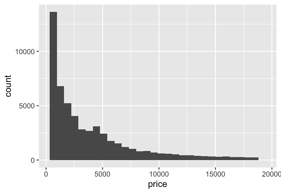

It’s heavily right-skewed: most diamonds are under $5,000. SO:

ggplot(diamonds,aes(x = price)) +
  geom_histogram(binwidth = 100) + 
  coord_cartesian(xlim = c(0,5000))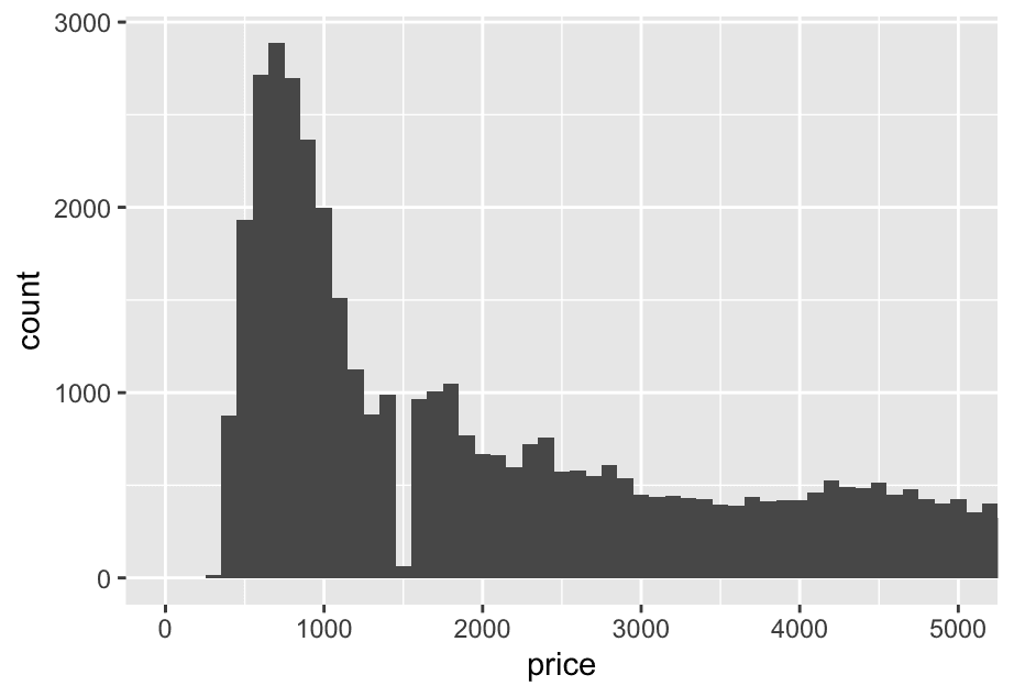

2. How many diamonds are 0.99 carat? How many are 1 carat? What do you think is the cause of the difference?

diamonds %>% 
  filter(carat == 0.99 | carat == 1) %>% 
  count(carat)

See it visually

ggplot(diamonds, aes(x = carat)) +
  geom_histogram(binwidth = 0.01) +
  coord_cartesian(xlim = c(0.95,1.05))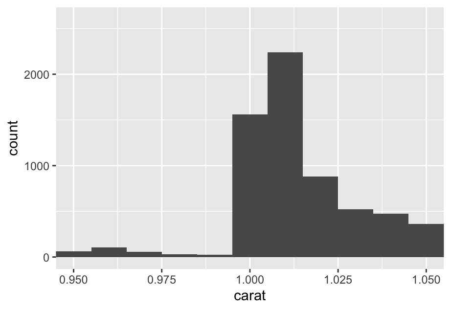

10.4 Unusual values

If you’ve encountered unusual values in your dataset, and simply want to move on to the rest of your analysis, you have two options.

1. Drop the entire row with the strange values:

diamonds2 <- diamonds %>% 
  filter(between(y,3,20))
  # only keep the rows where the `y` value is between 3 and 20 (inclusive).

We don’t recommend this option because one invalid value doesn’t imply that all the other values for that observation are also invalid. 2. Instead, we recommend replacing the unusual values with missing values. The easiest way to do this is to use mutate() to replace the variable with a modified copy. You can use the if_else() function to replace unusual values with NA`:

diamonds2 <- diamonds %>% 
  mutate(y = if_else(y < 3 | y > 30, NA, y))

y = if_else(condition, NA, y) If condition is TRUE, replace with NA; otherwise, keep original y. If the diamond’s width is less than 3 or more than 30, mark it as missing (NA).

It’s not obvious where you should plot missing values, so ggplot2 doesn’t include them in the plot, but it does warn that they’ve been removed:

> ggplot(diamonds2,aes(x = x, y = y)) +
+   geom_point()
Warning message:
Removed 9 rows containing missing values or values outside the scale range (`geom_point()`). 

To suppress that warning, set na.rm = TRUE:

ggplot(diamonds2,aes(x = x, y = y)) +
  geom_point(na.rm = TRUE)

Other times you want to understand what makes observations with missing values different to observations with recorded values. For example, in nycflights13::flights, missing values in the dep_time variable indicate that the flight was cancelled. So you might want to compare the scheduled departure times for cancelled and non-cancelled times. You can do this by making a new variable, using is.na() to check if dep_time is missing.

nycflights13::flights %>% 
  mutate(
    cancelled = is.na(dep_time),
    sched_hour = sched_dep_time %/% 100,
    sched_min = sched_dep_time  y`: Modulus (remainder)
 
This gives you what’s **left over** after the division.
Example:  
`515  100,
    sched_dep_time = sched_hour + (sched_min / 60)
  ) %>% 
  ggplot(aes(x = sched_dep_time)) +
  geom_freqpoly(aes(color = cancelled),binwidth = 1/4) +
  facet_wrap(~cancelled, scales = 'free_y')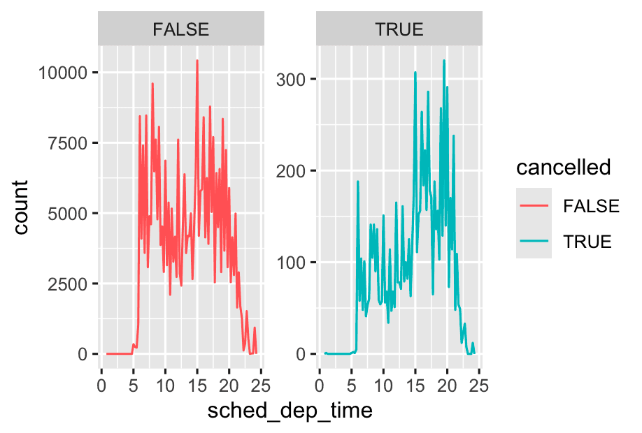 

• Use scales = "free_y" when group sizes are very different, but you want to compare shapes rather than absolute counts.

• Use default (scales = "fixed") when comparing absolute counts between groups is important

10.5 Covariation

Covariation is the tendency for the values of two or more variables to vary together in a related way. The best way to spot covariation is to visualize the relationship between two or more variables.

10.5.1 A categorical and a numerical variable

let’s explore how the price of a diamond varies with its quality (measured by cut) using geom_freqpoly()

ggplot(diamonds, aes(x = price)) +
  geom_freqpoly(aes(color = cut))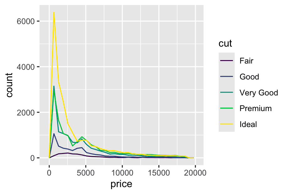

To make the comparison easier we need to swap what is displayed on the y-axis. Instead of displaying count, we’ll display the density, which is the count standardized so that the area under each frequency polygon is one.

ggplot(diamonds, aes(x = price, y = after_stat(density))) +
  geom_freqpoly(aes(color = cut))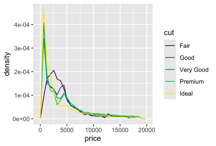

This makes it easier to compare the shapes of the distributions between groups, even if group sizes are very different.

Why is this important?

• If you have unequal group sizes (e.g., way more “Ideal” than “Fair”), plotting raw counts would make the big groups dominate the plot.

• By plotting density, you focus on the shape of each group’s price distribution, not just the total counts.

We see much less information about the distribution, but the boxplots are much more compact so we can more easily compare them (and fit more on one plot). It supports the counter-intuitive finding that better quality diamonds are typically cheaper!

ggplot(diamonds,aes(x = cut, y = price)) +
  geom_boxplot()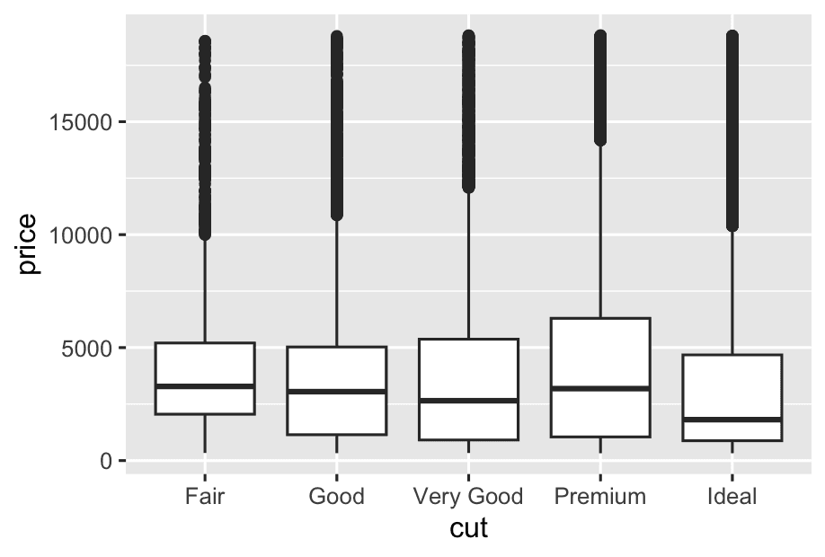

Take the class variable in the mpg dataset. You might be interested to know how highway mileage varies across classes:

ggplot(mpg, aes(x = class, y = hwy)) +
  geom_boxplot()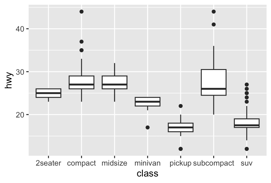

To make the trend easier to see, we can reorder class based on the median value of hwy:

ggplot(mpg, aes(x = fct_reorder(class, hwy, median), y = hwy)) +
  geom_boxplot()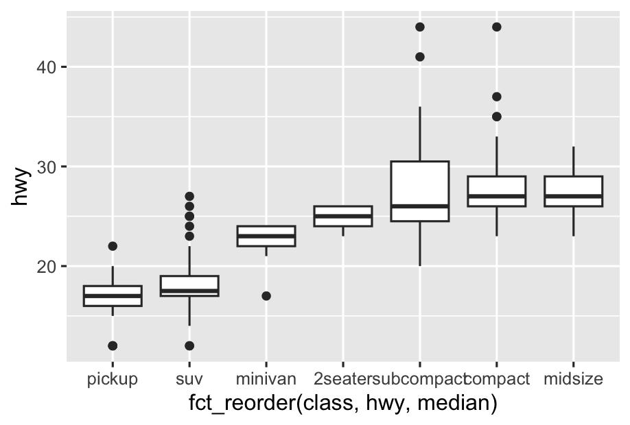

How does it work?

• For each class, calculate the median hwy.

• Reorder the class categories from lowest to highest median hwy.

If you have long variable names, geom_boxplot()] will work better if you flip it 90°. You can do that by exchanging the x and y aesthetic mappings.

ggplot(mpg, aes(x = hwy, y = fct_reorder(class, hwy, median))) +
  geom_boxplot()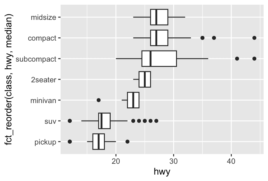

10.5.1.1 Exercises

Instead of exchanging the x and y variables, add coord_flip() as a new layer to the vertical boxplot to create a horizontal one. How does this compare to exchanging the variables?

p <- ggplot(mpg, aes(x = class, y =hwy)) +
  geom_boxplot()
p + coord_flip()

# Vertical boxplot (categories on x-axis, values on y-axis)
ggplot(mpg, aes(x = class, y = hwy)) +
  geom_boxplot()
 
# Swapped to horizontal (categories on y-axis, values on x-axis)
ggplot(mpg, aes(x = hwy, y = class)) +
  geom_boxplot()

For most simple boxplots, bar charts, etc.,

• Swapping x and y or using coord_flip() gives the same result visually.

But for more complex plots (e.g., certain geoms or coordinate systems),

• The statistical calculation always happens before coord_flip(),