Thought:
I found the book < r for data science> is confusing for, I need a small project to refine the skills, so I asked Chatgpt to create one for, guide me step by step, to help me better understand.
1. Explore the Dataset
What does mpg contain?
?mpg
How many rows and columns?
nrow(mpg) and ncol(mpg), or dim(mpg).
What are the key variables?
names(mpg) or str(mpg)
Glimpse at variable types and some sample rows.
glimpse(mpg)
2. Visualize Key Relationships
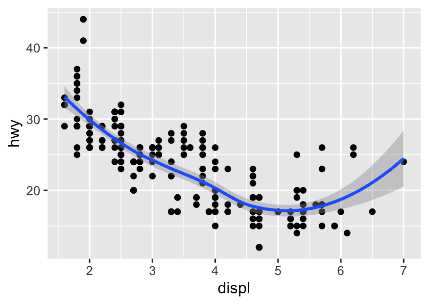
Step 1 The relationship between engine displacement and high-speed fuel consumption
library(ggplot2)

ggplot(mpg, aes(x = displ, y = hwy)) +
  geom_point() +
  geom_smooth()
-
What happens if you run only this line?
ggplot(mpg, aes(x = displ, y = hwy))What do you see? Empty plot. That’s because it’s just the canvas; we haven’t told ggplot how to draw yet. -
Why do we use
aes()insideggplot()? What does it actually do? Think ofaes()as “a mapping guide”aes()doesn’t draw anything by itself — it just tells the geoms (like points, lines, bars…) which variables to use when they eventually draw.So:
ggplot(data, aes(...))= “Here’s my dataset and how I want to map variables to visual features like x, y, color, size…” -
Why does
aes()not immediately create a legend, axis, or shape? What is it waiting for? Because you haven’t told it what shape to draw — e.g., points (geom_point()), lines (geom_line()), bars (geom_bar()), etc.
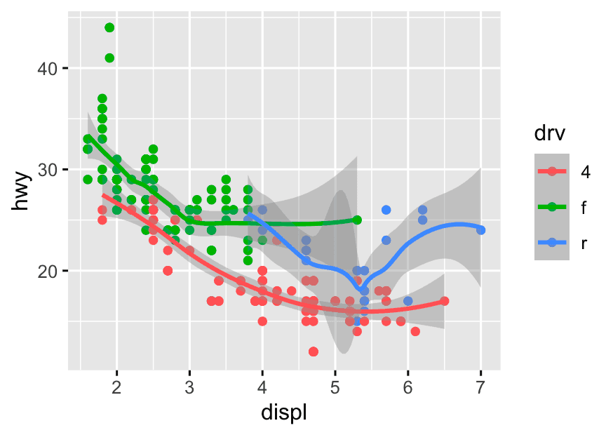
Step 2 Add Color to Show a Categorical Variable
ggplot(mpg, aes(x = displ, y =hwy, color = drv)) +
  geom_point() +
  geom_smooth()
Mapping color to a category lets you compare trends within subgroups, not just overall.
Step 3 Compare the relationship between engine size and fuel economy for each drive type (drv)
ggplot(mpg, aes(x = displ, y =hwy, color = drv)) +
  geom_point() +
  facet_wrap(~drv)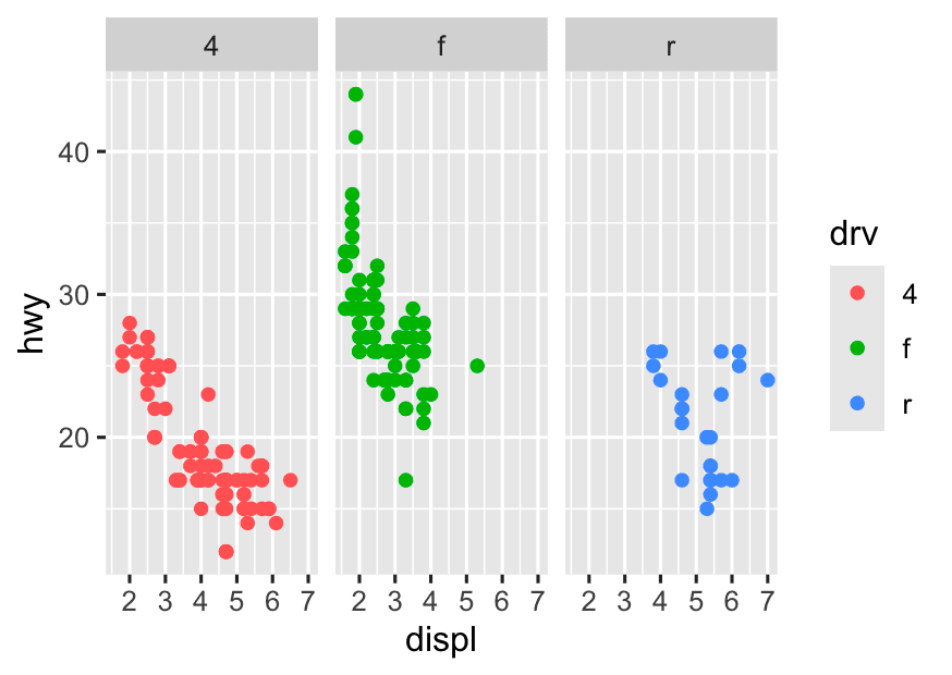
-
Single plot with color:
-
All points together, colored by group.
-
Trend lines can be drawn for each group, but it can get visually crowded, and overlapping points may obscure patterns.
-
-
Faceted plot:
-
Each group gets its own “mini-plot.”
-
Much easier to compare the trend and spread within each group, and spot differences.
-
No visual clutter or overlap between groups.
-
3 Summarize Data with dplyr
1. What is the average highway mpg for each car class?
mpg %>%
  group_by(class) %>%
  summarise(
    avg_hwy = mean(hwy, na.rm = TRUE)
  )
2. How many cars are there in each class?
count(mpg,class)
This is shorthand for: mpg %>% group_by(class) %>% summarise(n = n())
3. Which drive type (drv) is most common?
mpg %>%
  count(drv, sort = TRUE)
4. Which class has the highest average highway mpg?
mpg %>%
  group_by(class) %>%
  summarise(
    avg_hwy = mean(hwy, na.rm = TRUE)
  ) %>%
  arrange(desc(avg_hwy))
5.Who makes the most fuel-efficient SUVs?
mpg %>%
  filter(class == 'suv') %>%
  group_by(manufacturer) %>%
  summarise(avg_hwy = mean(hwy, na.rm = TRUE)) %>%
slice_max(avg_hwy)- Filter to only SUV-class cars.
- Reduces the dataset to relevant vehicles.
- Group by
manufacturer.- This splits the SUVs by who makes them.
- Summarise: For each manufacturer, calculate the average highway mpg (
avg_hwy).- Shows typical fuel economy by brand.
- Find the top(s): Use
slice_max()to get the manufacturer(s) with the highest average.- Alternatively, use
arrange(desc(avg_hwy))to list all in order.
- Alternatively, use
4 Visualize Summarized Data
1. Use dplyr to calculate average mpg by class.
mpg1 <- mpg %>%
  group_by(class) %>%
  summarise(
    avg_hwy = mean(hwy, na.rm = TRUE)
  )
ggplot(mpg1,aes(x = reorder(class, avg_hwy), y = avg_hwy)) +
geom_bar(stat = "identity")-
Used
reorder(class, avg_hwy)to sort the bars by average mpg. -
Used
geom_bar(stat = "identity")to make the bar heights reflect the avg value (you could also usegeom_col()).
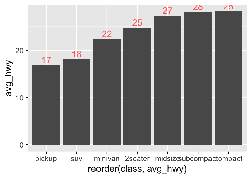
2. Add Value Labels on Bars
Show the exact average mpg on each bar for easier reading.
mpg1 <- mpg %>%
  group_by(class) %>%
  summarise(
    avg_hwy = mean(hwy, na.rm = TRUE)
  )
ggplot(mpg1,aes(x = reorder(class, avg_hwy), y = avg_hwy)) +
  geom_bar(stat = "identity") +
  geom_text(
    aes(label = round(avg_hwy),color = "pink"),
    vjust = -0.3
  ) +
  theme(legend.position = "none")
-
You can use
round(avg_hwy, 1)for one decimal place. -
Try
vjust = 1.2to put the label inside the bar, orvjust = -0.2to put it just above
Or you can use geom_label().
ggplot(mpg1, aes(x = reorder(class, avg_hwy), y = avg_hwy)) +
  geom_bar(stat = "identity") +
  geom_label(
    aes(label = round(avg_hwy, 1)),  # Label inside box
    vjust = -0.3,                    # Controls vertical position
    fill = "white",                  # Box background (optional)
    color = "black"                  # Text color (optional)
  ) +
  theme(legend.position = "none")
3. Compare Two Variables: Grouped or Colored Bars
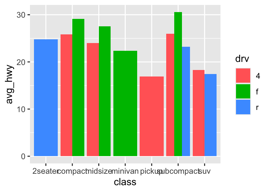
- For example: Compare average
hwyby bothclassanddrv(drive type).
mpg %>%
  group_by(class, drv) %>%
  summarise(avg_hwy = mean(hwy, na.rm = TRUE)) %>%
  ggplot(aes(x = class, y = avg_hwy, fill = drv)) +
geom_bar(stat = "identity", position = "dodge")- For grouped/colored bar charts (e.g., avg mpg by class & drv), always use group_by() + summarise() first.
4. Visualize Counts (Number of Cars) Instead of Averages**
- Make a bar chart showing how many cars are in each class.
mpg %>%
  group_by(class, drv) %>%
  ggplot(aes(x = class, fill = drv)) +
  geom_bar(position = "dodge")
# this is not the best answer- Does group_by() matter here?
-
In this case,
group_by()is unnecessary. -
geom_bar()(by default) counts the number of rows in each group automatically based on what’s mapped inaes().
- How does ggplot2 count?
-
If you don’t set
stat = "identity",geom_bar()will:-
Count the number of observations for each
xvalue (here, eachclass) -
When you add
fill = drv, it will split each bar bydrv, and withposition = "dodge"the bars for differentdrvin the same class will be side-by-side.
-
- What happens if you use
group_by()before ggplot?
-
In this situation,
group_by()has no effect—ggplot2 does its own internal grouping and counting. -
So you can skip
group_by()completely. -
When visualizing counts (e.g., how many cars in each class, split by drv), you do NOT need to pre-summarize or group_by()—just map x and fill, and let geom_bar() do the counting.
-
Only use group_by() + summarise() when you want to compute your own summary statistics (mean, median, etc.).
-
For counts, this is enough:
  ggplot(mpg, aes(x = class, fill = drv)) +
    geom_bar(position = "dodge")
5 Explore Trends Over Another Variable
-
If you’re curious: “Does average mpg change by number of cylinders (
cyl) or manufacturer?” -
Summarize by that variable and plot.
-
If you want to compare means/averages
(e.g., “What is the average highway mpg for each cylinder group?”)
👉 Use a summary table and plot with a bar chart, point plot, or line plot.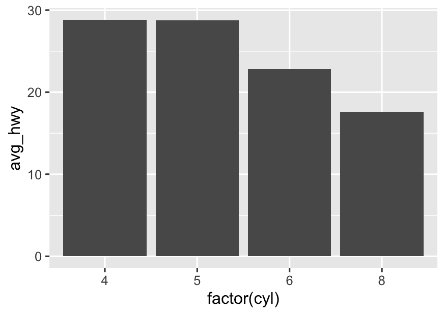
mpg %>%
  group_by(cyl) %>%
  summarise(avg_hwy = mean(hwy, na.rm = TRUE)) %>%
  ggplot(aes(x = factor(cyl),y = avg_hwy)) +
geom_col()- If you want to compare distributions
(e.g., “What does the distribution of highway mpg look like for each cylinder group?”)
👉 Use the original (raw) data and plot withgeom_freqpoly(),geom_histogram(), or boxplots.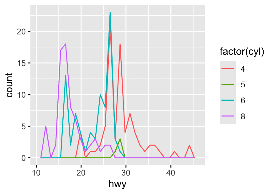
ggplot(mpg,aes(x = hwy, color = factor(cyl))) +
geom_freqpoly()-
Summary tables are for visualizing summaries (means, medians) with one value per group.
-
Raw data is for visualizing the shape of the data (distribution) across groups.
-
Use summarized data for summaries;
-
Use raw data for distribution plots.
6 Polish the Chart for Publication/Presentation
Challenge 1: Add a custom color palette.
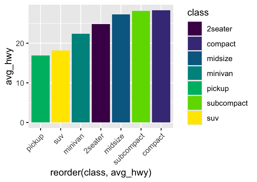
mpg1 <- mpg %>%
  group_by(class) %>%
  summarise(avg_hwy = mean(hwy, na.rm = TRUE))

library(viridis)
ggplot(mpg1, aes(x = reorder(class, avg_hwy), y = avg_hwy, fill = class)) +
  geom_col() +
  scale_fill_viridis_d() +
  theme(axis.text.x = element_text(angle = 45,hjust=1))
Use theme(axis.text.x = element_text(angle = X)) in ggplot2 to control the rotation of x-axis labels.
Adjust hjust and vjust as needed for best alignment.
Challenge 2: Make the labels prettier (e.g., use scales::comma for big numbers).
Step 1: Introducing the scales package
-
The
scalespackage is part of the tidyverse and specializes in making numbers pretty for plots. -
It gives you handy functions like:
-
comma()(adds thousand separators: 10,000) -
dollar()(adds 10,000) -
percent()(turns 0.32 into 32%)
-
Step 2: How does ggplot2 use these formatting functions?
-
ggplot2’s axis functions (
scale_x_continuous,scale_y_continuous) can take alabels =argument. -
You pass in a formatting function—like
comma—and ggplot2 will automatically use it for the axis tick labels.
Example logic (not code):
-
“For my y-axis, I want the numbers to look like 12,000 not 12000.”
-
So, in my y-axis scale, I’ll set
labels = comma.
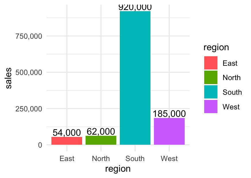
Example 1: Formatting “Population” or “Sales”
Suppose you have a table of total sales (in dollars) by region:
library(dplyr)
library(ggplot2)
library(scales)

sales <- tibble::tribble(
  ~region,    ~sales,
  "East",     54000,
  "West",     185000,
  "North",    62000,
  "South",    920000
)

ggplot(sales, aes(x = region, y = sales, fill = region)) +
  geom_col() +
  geom_text(aes(label = comma(sales)), vjust = -0.2) +   # Adds comma to label above bar
  scale_y_continuous(labels = comma) +                   # Adds comma to y-axis numbers
  theme_minimal()
What you’ll see:
-
Y-axis: 920,000 instead of 920000
-
Value labels above bars: 54,000, 185,000, etc.
Example 2: Using dollar() for Currency
If those sales numbers are in dollars, you can use:
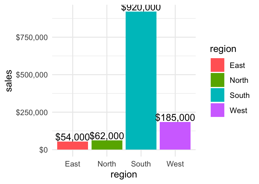
ggplot(sales, aes(x = region, y = sales, fill = region)) +
  geom_col() +
  geom_text(aes(label = dollar(sales)), vjust = -0.2) +  # $920,000
  scale_y_continuous(labels = dollar) +                  # $ on axis
  theme_minimal()
Example 3: Using percent() for Rates
Suppose you have conversion rates:
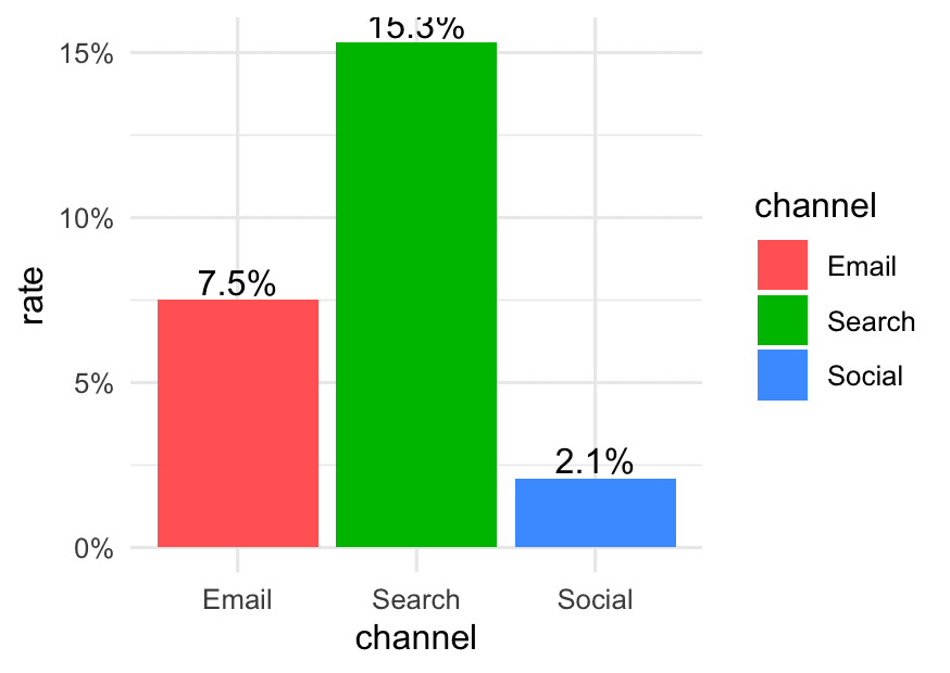
conversion <- tibble::tribble(
  ~channel,  ~rate,
  "Email",   0.075,
  "Social",  0.021,
  "Search",  0.153
)

ggplot(conversion, aes(x = channel, y = rate, fill = channel)) +
  geom_col() +
  geom_text(aes(label = percent(rate)), vjust = -0.2) +
  scale_y_continuous(labels = percent) +
  theme_minimal()
Effect:
- Shows labels and axis as 7.5%, 2.1%, 15.3%
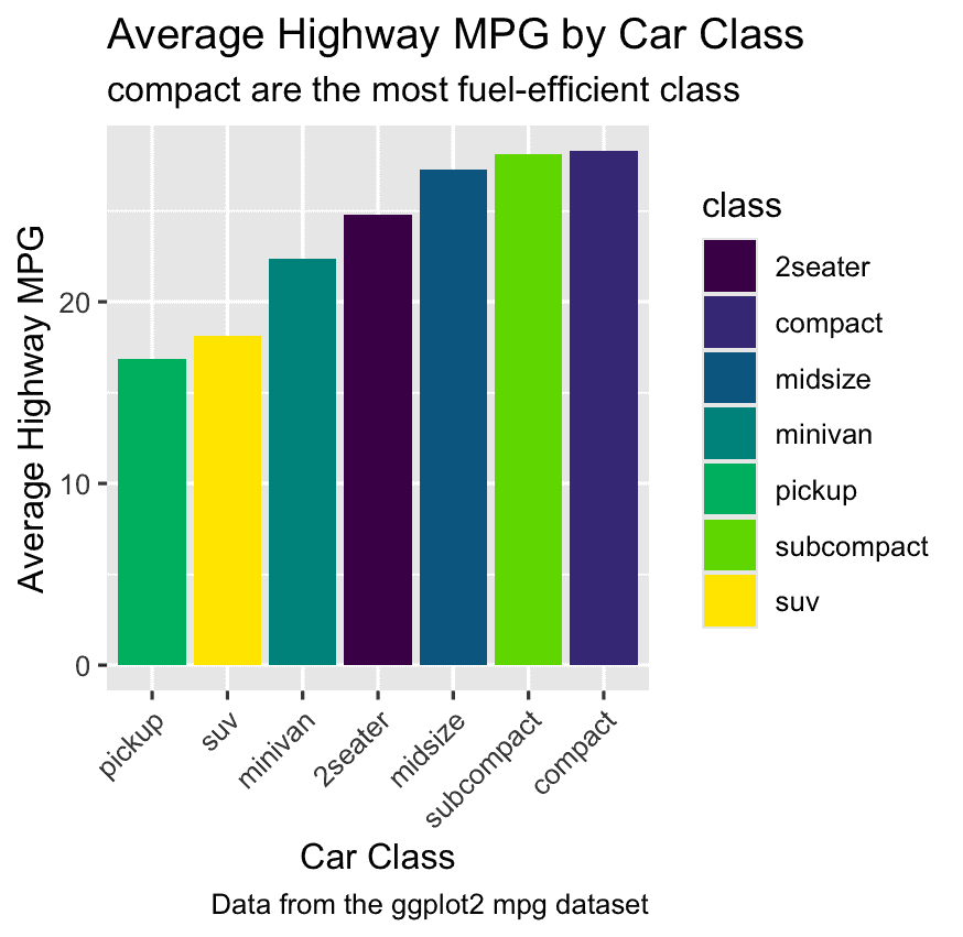
Challenge 3: Add a chart caption
Find the most fuel-efficient class:
# 1. Summarize the data
mpg_summary <- mpg %>%
  group_by(class) %>%
  summarise(avg_hwy = mean(hwy, na.rm = TRUE))

# 2. Find the most fuel-efficient class
top_class <- mpg_summary %>%
  slice_max(avg_hwy) %>%
  pull(class)

# 3. Create the subtitle string
subtitle_var <- paste0(top_class, " are the most fuel-efficient class")

# 4. Create the plot
ggplot(mpg_summary, aes(x = reorder(class, avg_hwy), y = avg_hwy, fill = class)) +
  geom_col() +
  scale_fill_viridis_d() +
  labs(
    title    = "Average Highway MPG by Car Class",
    subtitle = subtitle_var,
    x        = "Car Class",
    y        = "Average Highway MPG",
    caption  = "Data from the ggplot2 mpg dataset"
  ) +
  theme(axis.text.x = element_text(angle = 45, hjust = 1))